-------------------------------------------------------------------------------
What is an Agent Based Model?
-------------------------------------------------------------------------------


                       Example: The spread of a disease


    In this model each agent can be in one of three states:


        Susceptible: the agent is healthy, but can get the disease.
        Infectious: the agent has the disease and can spread it to others.
        Recovered: the agent has had the disease and is now immune.


    In the first round one or more agents get infected.


    In all subsequent rounds:


        - All infectious agents have a chance to become recovered, and
        - all recovered agents get a chance to become susceptible.
        - All agents that are still infectious contact a random number of
        other agents
        - Each of these contact has a chance of resulting in an infection if
        someone is susceptible.

. set seed 123456789


. set scheme s1color


. clear mata


. drop _all


. run sir_main.do


. 
. mata:
------------------------------------------------- mata (type end to exit) -----
: 
: model = sir()


: model.N(2000)


: model.tdim(150)


: model.outbreak(5)


: model.mcontacts(4)


: model.transmissibility(0.045)


: model.mindur(10)


: model.meandur(14)


: model.pr_loss(0)


: model.run()
----+--- 1 ---+--- 2 ---+--- 3 ---+--- 4 ---+--- 5
..................................................        50
..................................................       100
..................................................       150


: model.export_sir()


: end
-------------------------------------------------------------------------------


. 
. twoway line S I R t,  name(sir1, replace)          ///
>    ylabel(,angle(0)) legend(rows(1)) lwidth(*1.5 ..) 


.    
. drop _all

    The number 0.045 for transmissibility was chosen to get a >> R0of
    2.5, which in line with COVID-19.


 
-------------------------------------------------------------------------------

<< index >>

-------------------------------------------------------------------------------

-------------------------------------------------------------------------------
What is an Agent Based Model?
-------------------------------------------------------------------------------


                               Adding a network


    The model thus far does not need a simulation; one can compute them with
    a set of differential equations.


    In Stata you can do that with epimodels by Sergiy Radyakin and Paolo
    Verme


    However, the advantage of Agent Based Models is that it is much easier to
    expand the model.


    For example, what if we don't believe that people contact each other
    randomly but instead it is a network that determines who contacts who.


    A common model that works fairly well for a lot of social networks is a
    small world network:


        We assume all agents are on a circle, and that each agent is
        connected to the 4 closes agents.


        However, a small number of these connections are replaced by a
        connection to a random agent

. clear mata


. set seed 28863


. run nw_main.do


. mata:
------------------------------------------------- mata (type end to exit) -----
: model = sir_nw()


: model.N(100)


: model.tdim(10)


: model.outbreak(2)


: model.degree(4)


: model.pr_long(.05)


: model.transmissibility(0.1)


: model.mindur(5)


: model.meandur(6)


: model.pr_loss(0.00)


: model.run()
----+--- 1 ---+--- 2 ---+--- 3 ---+--- 4 ---+--- 5
..........
: model.export_nw()


: end
-------------------------------------------------------------------------------


. 
. gen x_ego = cos((ego-1)/`n'*2*_pi)*(1+mod(ego,2)*.2)


. gen y_ego = sin((ego-1)/`n'*2*_pi)*(1+mod(ego,2)*.2)


. gen x_alter = cos((alter-1)/`n'*2*_pi)*(1+mod(alter,2)*.2)
(1 missing value generated)


. gen y_alter = sin((alter-1)/`n'*2*_pi)*(1+mod(alter,2)*.2)
(1 missing value generated)


.     
. 
. bys ego (alter) : gen first = _n == 1


. 
. forvalues t = 1/10{
  2.     twoway pcspike y_ego x_ego y_alter x_alter,                ///
>                   lcolor(gs8)                               || ///
>         scatter y_ego x_ego if first & state`t'==1 ,           ///
>                    mcolor(yellow) msymbol(O)                || ///
>         scatter y_ego x_ego if first & state`t'==2 ,           ///
>                    mcolor(red) msymbol(O)                   || ///
>         scatter y_ego x_ego if first & state`t'==3 ,           ///
>                    mcolor(black) msymbol(Oh)                   ///         
>                    aspect(1) xscale(off) yscale(off)           ///
>                    legend(order(2 "infected"                   ///
>                                 3 "susceptible"                ///
>                                 4 "recovered") rows(1))        ///
>                    name(t`t', replace) title(Time `t')     
  3. }


. drop _all

    Close knit networks tend to slow down the spread of a disease, while the
    long distance ties tend


    So that is one way in which advise against unnecesary travel or "social
    buble" rules in countries like Belgium works


 
-------------------------------------------------------------------------------

<< index >>

-------------------------------------------------------------------------------

-------------------------------------------------------------------------------
How to implement an ABM in Mata
-------------------------------------------------------------------------------


                                Basic SIR model


    Lets take a look at the code for the basic SIR model:

version 16.1

run abm_pop.mata

mata:

mata set matastrict on

class sir {
	class abm_pop          scalar agents
	
	real                   scalar tdim
	real                   scalar outbreak
	real                   scalar removed
	real                   scalar mcontacts
	real                   scalar N
	real                   scalar transmissibility
	real                   scalar mindur
	real                   scalar meandur
	real                   scalar pr_heal
	real                   scalar pr_loss
	
	// sir_chks.do
	void                          posint()
	void                          pr()
	void                          isid()
	void                          istime()
	
	// sir_set_pars.do
	transmorphic                  N()
	transmorphic                  tdim()
	transmorphic                  outbreak()
	transmorphic                  removed()
	transmorphic                  mcontacts()
	transmorphic                  transmissibility()
	transmorphic                  mindur()
	transmorphic                  meandur()
	transmorphic                  pr_loss()

	// sir_sim.do
	void                          setup()
	real                   matrix meet()
	real                   scalar infect()
	void                          progress()
	void                          step()
	void                          run()
	void                          dots()
	
	// sir_export.do
	void                          export_sir()
	void                          export_r()
}
end 

do sir_chks.do
do sir_set_pars.do
do sir_sim.do
do sir_export.do

exit

    The model is implemented as a >> class


    The population is stored is stored in another class abm_pop, which is
    available from https://github.com/maartenteaches/abm_pop.


    Whatever is stored in abm_pop is assumed to persist until you store
    something else. So you only have to store the disease state of an agent
    when it changes. This can save a lot of reading and writing and make the
    simulation run quicker.


    There are various checks perfomed and we can see those

include sir_locals.do

mata:
void sir::posint(real scalar val)
{
	if (val <= 0 | val != ceil(val)) {
		_error("argument must be a positive integer")
	} 
}

void sir::pr(real scalar val)
{
	if (val <0 | val > 1) {
		_error("argument must be between 0 and 1")
	}
}

void sir::isid(real scalar id)
{
	if (id < 0 | id > N | id!=ceil(id)) {
		_error("argument is not a valid id")
	}
	
}

void sir::istime(real scalar t)
{
	if (t<0 | t > tdim | t!=ceil(t)) {
		_error("argument is not a valid time")
	}
}
end

    The functions that set the parameters are shown

include sir_locals.do

mata:

transmorphic sir::N(| real scalar val)
{
	if (args() == 1) {
		posint(val)
		N = val
	}
	else {
		return(N)
	}
}

transmorphic sir::tdim(| real scalar val)
{
	if (args() == 1) {
		posint(val)
		tdim= val
	}
	else {
		return(tdim)
	}
}


transmorphic sir::outbreak(| real scalar val)
{
	if (args() == 1) {
		posint(val)
		outbreak= val
	}
	else {
		return(outbreak)
	}
}

transmorphic sir::removed(| real scalar val)
{
	if (args() == 1) {
		posint(val)
		removed= val
	}
	else {
		return(removed)
	}
}

transmorphic sir::mcontacts(| real scalar val)
{
	if ( args()==1 ) {
		if ( val < 0) _error("arguments must be positive")
		mcontacts = val
	}
	else {
		return(mcontacts)
	}
}

transmorphic sir::transmissibility(| real scalar val)
{
	if ( args()==1 ) {
		pr(val)
		transmissibility = val
	}
	else {
		return(transmissibility)
	}
}

transmorphic sir::mindur(| real scalar val)
{
	if ( args()==1 ) {
		posint(val)
		mindur = val
	}
	else {
		return(mindur)
	}
}

transmorphic sir::meandur(| real scalar val)
{
	if ( args()==1 ) {
		if (val < 0) _error("argument must be positive")
		meandur = val
	}
	else {
		return(meandur)
	}
}

transmorphic sir::pr_loss(| real scalar val)
{
	if ( args()==1 ) {
		pr(val)
		pr_loss = val
	}
	else {
		return(pr_loss)
	}
}


end

    The main simulation functions are

include sir_locals.do

mata:

void sir::run()
{
	real scalar i, t
	setup()

	dots(0)
	dots(1)

	for (t=2; t<=tdim; t++) {
		dots(t)
		for(i=1; i<=N ; i++) {
			step(i,t)
		}
	}
}

void sir::setup()
{
	real vector id, key
	real scalar i
	
	if (N==.)                   _error("N has not been set")
	if (tdim==.)                _error("tdim has not been set")
	if (outbreak==.)            _error("outbreak has not been set")
	if (outbreak > N)           _error("the initial outbreak is larger than population")
	if (removed==.)             removed = 0
	if (removed + outbreak > N) _error("intial outbreak + removed agents is larger than the population")
	if (mcontacts==.)           _error("mcontacts has not been set")
	if (mcontacts > N)          _error("average number of mcontacts is larger than population")
	if (transmissibility==.)    _error("transmissibility has not been set")
	if (mindur==.)              _error("mindur has not been specified")
	if (meandur==.)             _error("meandur has not been specified")
	if (meandur <= mindur)      _error("meandur must be larger than mindur")
	if (pr_loss==.)             pr_loss = 0
	
	agents.N(N)
	agents.k(3)
	agents.setup()
	
	id = jumble((1..N)')
	
	for (i = 1; i<= N; i++) {
		key = id[i],`state',1
		agents.put(key,(i<=outbreak ? `infectious' : (i <= outbreak+removed ? `removed' : `susceptible')))
		key[2] = `exposes'
		if (i <= outbreak) agents.put(key, J(2,0,.) )
		
		key[2] = `dur'
		agents.put(key,1)
	}

	
// if meandur - mindur < 1 then pr_heal > 1, so there is no randomness to the duration
// and the fixed duration of the disease is mindur	
	pr_heal = 1/(meandur-mindur)
}

void sir::step(real scalar id, real scalar t)
{
	real matrix exposed
	real scalar i, k
	real rowvector key
	
	isid(id)
	istime(t)

	key = id, `dur',t

	agents.put(key, agents.get(key, "last")+1)
	progress(id,t)
	key = id, `state',t
	if (agents.get(key, "last") == `infectious' ) {
		exposed = meet(id, t)
		for(i=1; i<= cols(exposed); i++) {
			exposed[2,i] = infect(exposed[1,i],t) 
		}
		key[2] = `exposes'
		agents.put(key,exposed)
	}
}

void sir::progress(real scalar id, real scalar t)
{
    real rowvector key1, key2, key3
	
	isid(id)
	istime(t)
	
	key1 = id, `state',t
	key2 = id, `dur',t
	if (agents.get(key1, "last") == `infectious'  & agents.get(key2, "last") > mindur) {
		if (runiform(1,1) < pr_heal) {
			agents.put(key1, `removed')
			agents.put(key2,1)
			key3 = id, `exposes',t
			agents.put(key3,NULL)
		}
	}
    if (agents.get(key1, "last") == `removed' & runiform(1,1) < pr_loss) {
		agents.put(key1, `susceptible')
		agents.put(key2,1)
	}
}

real matrix sir::meet(real scalar id, real scalar t)
{
	real scalar k
	real colvector res
	real rowvector key

	isid(id)
	
	k = rpoisson(1,1,mcontacts)
	if (k == 0) {
		return(J(2,0,.))
	}
	else{
		res =  ceil(runiform(1,k):*(N-1))
		res = res + (res:>=id)
		res = res \ J(1,k,.)
		return (res)
	}
}

real scalar sir::infect(real scalar id, real scalar t)
{
	real vector key
	real scalar infected

	isid(id)
	istime(t)

	infected = 0
	key = id,`state', t
	if (agents.get(key, "last")==`susceptible') {
		if (runiform(1,1) < transmissibility) {
			agents.put(key, `infectious')
			key[2] = `dur'
			agents.put(key, 1)
			key[2] = `exposes'
			agents.put(key,J(2,0,.))
			infected = 1
		}
	}
	return(infected)
}



void sir::dots(real scalar t) 
{
	if (t==0) {
		printf("----+--- 1 ---+--- 2 ---+--- 3 ---+--- 4 ---+--- 5\n")
	}
	else if (mod(t, 50) == 0) {
		printf(". %9.0f\n", t)
	}
	else {
		printf(".")
	}
	displayflush()
}
end

    The "variables" in agents are actually numbered and not named. To make it
    easier to read the code I use local macros defined in

// address in abm_pop class agents
local state       = 1
local dur         = 2
local exposes     = 3

// states
local susceptible = 1
local infectious  = 2 
local removed     = 3

    The functions that allow you to export the results to Stata are

include sir_locals.do

mata:

void sir::export_sir(| string rowvector names)
{
    real matrix res
	pointer matrix p
    string rowvector varnames
	real scalar xid, n, i, j

	if (args() == 1) {
		if (cols(names)!= 4) _error("4 variable names need to be specified")
		varnames = names
	}
	else {
		varnames = "t", "S", "I", "R"
	}

	res = J(N,tdim,.)
	p = agents.extract(`state', tdim)
	for (i=1; i<=N; i++) {
		for(j=1; j<=tdim; j++) {
			res[i,j] = *p[i,j]
		}
	}
	res =  (1..tdim)', mean(res:==`susceptible')', 
	                   mean(res:==`infectious')', 
					   mean(res:==`removed')'

	xid = st_addvar("float", varnames)
    n = st_nobs()
    n = rows(res) - n
    if (n > 0) {
        st_addobs(n)
    }
    st_store(.,xid, res)
}

void sir::export_r()
{
	real matrix res
	pointer matrix p_exposes, p_state
	real scalar xid, n, i, j, t
	string rowvector varnames
	real colvector n_ill

	t = .
	
	res = (1..tdim)',J(tdim,1,0)
	n_ill = J(tdim,1,0)
	p_exposes = agents.extract(`exposes',tdim)
	p_state = agents.extract(`state',tdim)
	for (i=1; i<=N; i++) {
		if (*p_state[i,1]==`infectious') {
			t=1  
		} 
		else {
		    t=.
		}
		for(j=2;j<=tdim;j++) {
			if (*p_state[i,j-1]==`susceptible' & 
			    *p_state[i,j]  ==`infectious') {
					t=j
					n_ill[t] = n_ill[t] + 1
				}
			if (*p_state[i,j-1]==`infectious' & 
			    (*p_state[i,j]  ==`removed' | *p_state[i,j]  ==`susceptible')) t = .
			if (t!=.) {
			    res[t,2] = res[t,2] + rowsum((*p_exposes[i,j])[2,.])
			}
		}
	}
	res[.,2] = res[.,2]:/n_ill
	varnames = "t", "reprod"
    xid = st_addvar("float", varnames)
    n = st_nobs()
    n = rows(res) - n
    if (n > 0) {
        st_addobs(n)
    }
    st_store(.,xid, res)
	
}


end

 
 
-------------------------------------------------------------------------------

<< index >>

-------------------------------------------------------------------------------

-------------------------------------------------------------------------------
How to implement an ABM in Mata
-------------------------------------------------------------------------------


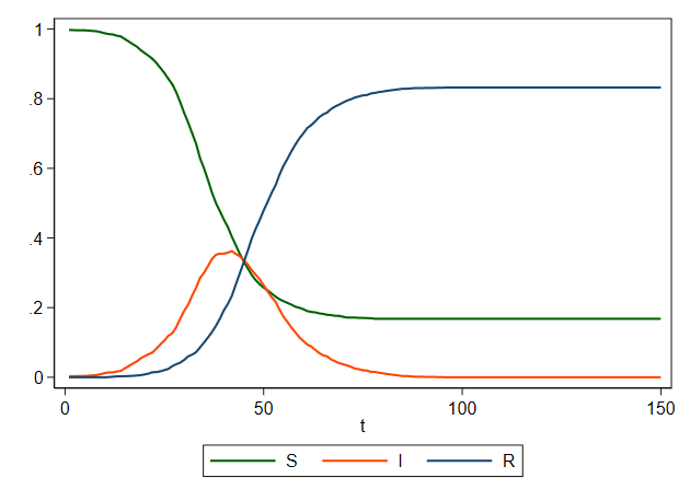
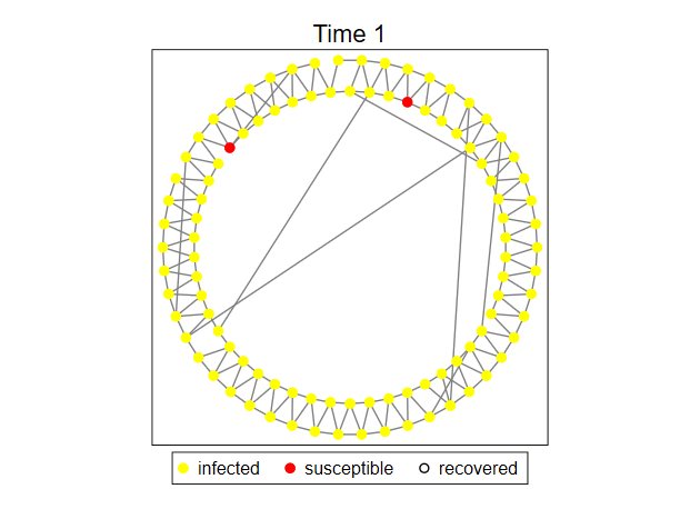
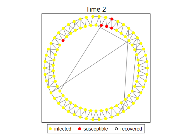
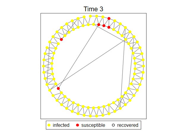
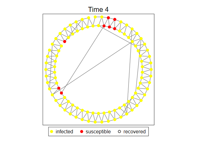
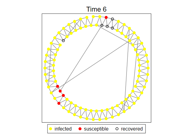
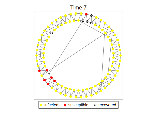
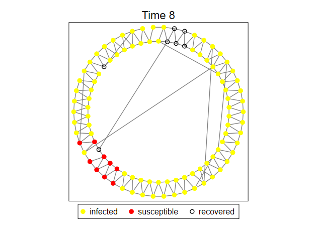
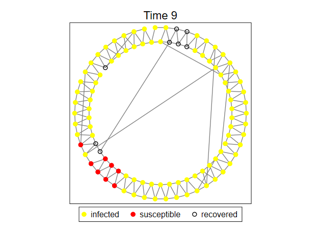
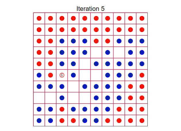
                            SIR model in a network


    To add the network we make use the abm_nw class, which is available from 
    https://github.com/maartenteaches/abm_nw.


    This takes care of creating the network and keeps track of who can
    contact who.


    With that the changes required are fairly small


    The class definition is

version 16.1

run abm_pop.mata
run abm_nw.mata                                          // <-- new

mata:

mata set matastrict on

class sir_nw {
	class abm_pop          scalar agents
	class abm_nw           scalar nw                     // <-- new
	
	real                   scalar tdim
	real                   scalar outbreak
	real                   scalar removed
//	real                   scalar mcontacts              // <-- no longer necessary
	real                   scalar N
	real                   scalar transmissibility
	real                   scalar mindur
	real                   scalar meandur
	real                   scalar pr_heal
	real                   scalar pr_loss
	real                   scalar degree                 // <-- new
	real                   scalar pr_long                // <-- new
	
	// sir_chks.do
	void                          posint()
	void                          pr()
	void                          isid()
	void                          istime()
	
	// sir_set_pars.do
	transmorphic                  N()
	transmorphic                  tdim()
	transmorphic                  outbreak()
	transmorphic                  removed()
//	transmorphic                  mcontacts()           // <-- no longer necessary
	transmorphic                  transmissibility()
	transmorphic                  mindur()
	transmorphic                  meandur()
	transmorphic                  pr_loss()
	transmorphic                  degree()              // <-- new
	transmorphic                  pr_long()             // <-- new

	// sir_sim.do
	void                          setup()
//	real                   matrix meet()                // <-- no longer necessary
	real                   scalar infect()
	void                          progress()
	void                          step()
	void                          run()
	void                          dots()
	
	// sir_export.do
	void                          export_sir()
	void                          export_r()
	void                          export_nw()          // <-- new
}
end 

do nw_chks.do
do nw_set_pars.do
do nw_sim.do
do nw_export.do

exit

    Checks and setting parameters are pretty much the same


    The main simulation functions are

include nw_locals.do

mata:

void sir_nw::run()
{
	real scalar i, t
	setup()

	dots(0)
	dots(1)

	for (t=2; t<=tdim; t++) {
		dots(t)
		for(i=1; i<=N ; i++) {
			step(i,t)
		}
	}
}

void sir_nw::setup()
{
	real vector id, key
	real scalar i
	
	if (N==.)                   _error("N has not been set")
	if (tdim==.)                _error("tdim has not been set")
	if (outbreak==.)            _error("outbreak has not been set")
	if (outbreak > N)           _error("the initial outbreak is larger than population")
	if (removed==.)             removed = 0
	if (removed + outbreak > N) _error("intial outbreak + removed agents is larger than the population")
	if (transmissibility==.)    _error("transmissibility has not been set")
	if (mindur==.)              _error("mindur has not been specified")
	if (meandur==.)             _error("meandur has not been specified")
	if (meandur <= mindur)      _error("meandur must be larger than mindur")
	if (pr_loss==.)             pr_loss = 0
	if (degree==.)              _error("degree has not been specified")  // <-- new
	if (pr_long==.)             _error("pr_long has not been specified") // <-- new
	
	nw.clear()                                                           // <-- new   
	nw.N_nodes(0,N)                                                      // <-- new
	nw.directed(0)                                                       // <-- new
	nw.tdim(0)                                                           // <-- new
	nw.sw(degree,pr_long)                                                // <-- new    
	nw.setup()                                                           // <-- new
	
	agents.N(N)
	agents.k(4)
	agents.setup()
	
	id = jumble((1..N)')
	
	for (i = 1; i<= N; i++) {
		key = id[i],`state',1
		agents.put(key,(i<=outbreak ? `infectious' : (i <= outbreak+removed ? `removed' : `susceptible')))
		key[2] = `exposes'
		if (i <= outbreak) agents.put(key, J(2,0,.) )
		
		key[2] = `dur'
		agents.put(key,1)
	}

	
// if meandur - mindur < 1 then pr_heal > 1, so there is no randomness to the duration
// and the fixed duration of the disease is mindur	
	pr_heal = 1/(meandur-mindur)
}

void sir_nw::step(real scalar id, real scalar t)
{
	real matrix exposed
	real scalar i, k
	real rowvector key
	
	isid(id)
	istime(t)

	key = id, `dur',t

	agents.put(key, agents.get(key, "last")+1)
	progress(id,t)
	key = id, `state',t
	if (agents.get(key, "last") == `infectious' ) {
		exposed = nw.neighbours(id)                        // <-- new
		exposed = exposed \ J(1,cols(exposed),.)           // <-- new
		for(i=1; i<= cols(exposed); i++) {
			exposed[2,i] = infect(exposed[1,i],t) 
		}
		key[2] = `exposes'
		agents.put(key,exposed)
	}
}

void sir_nw::progress(real scalar id, real scalar t)
{
    real rowvector key1, key2, key3
	
	isid(id)
	istime(t)
	
	key1 = id, `state',t
	key2 = id, `dur',t
	if (agents.get(key1, "last") == `infectious'  & agents.get(key2, "last") > mindur) {
		if (runiform(1,1) < pr_heal) {
			agents.put(key1, `removed')
			agents.put(key2,1)
			key3 = id, `exposes',t
			//agents.put(key3,NULL)
		}
	}
    if (agents.get(key1, "last") == `removed' & runiform(1,1) < pr_loss) {
		agents.put(key1, `susceptible')
		agents.put(key2,1)
	}
}

real scalar sir_nw::infect(real scalar id, real scalar t)
{
	real vector key
	real scalar infected

	isid(id)
	istime(t)

	infected = 0
	key = id,`state', t
	if (agents.get(key, "last")==`susceptible') {
		if (runiform(1,1) < transmissibility) {
			agents.put(key, `infectious')
			key[2] = `dur'
			agents.put(key, 1)
			key[2] = `exposes'
			agents.put(key,J(2,0,.))
			infected = 1
		}
	}
	return(infected)
}

void sir_nw::dots(real scalar t) 
{
	if (t==0) {
		printf("----+--- 1 ---+--- 2 ---+--- 3 ---+--- 4 ---+--- 5\n")
	}
	else if (mod(t, 50) == 0) {
		printf(". %9.0f\n", t)
	}
	else {
		printf(".")
	}
	displayflush()
}
end

 
 
-------------------------------------------------------------------------------

<< index >>

-------------------------------------------------------------------------------

-------------------------------------------------------------------------------
ancillary
-------------------------------------------------------------------------------


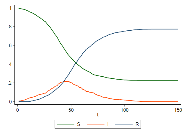
                                Other Scenarios


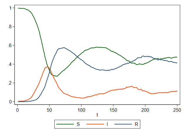
    Recently, there have an increasing number of news stories about that
    immunity against COVID-19 does not persist


    We can change to model to see how that impacts the spread of the disease

. clear mata


. drop _all


. run sir_main.do


. 
. mata:
------------------------------------------------- mata (type end to exit) -----
: 
: model = sir()


: model.N(2000)


: model.tdim(250)


: model.outbreak(5)


: model.mcontacts(4)


: model.transmissibility(0.045)


: model.mindur(10)


: model.meandur(14)


: model.pr_loss(0.02)


: model.run()
----+--- 1 ---+--- 2 ---+--- 3 ---+--- 4 ---+--- 5
..................................................        50
..................................................       100
..................................................       150
..................................................       200
..................................................       250


: model.export_sir()


: end
-------------------------------------------------------------------------------


. 
. twoway line S I R t,  name(anc1, replace)          ///
>    ylabel(,angle(0)) legend(rows(1)) lwidth(*1.5 ..) 


. drop _all

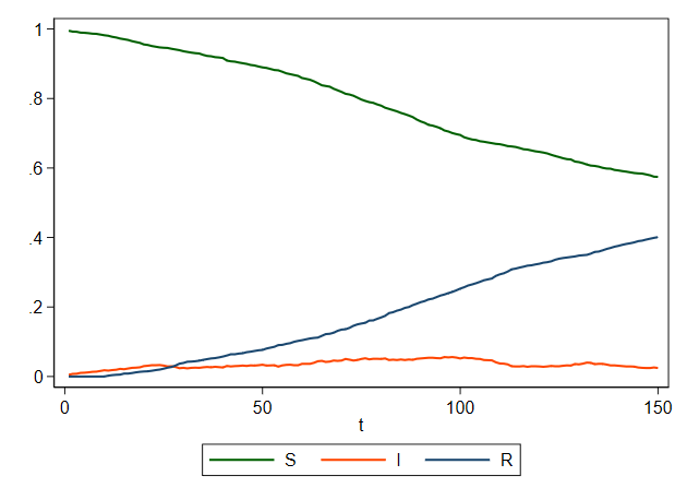
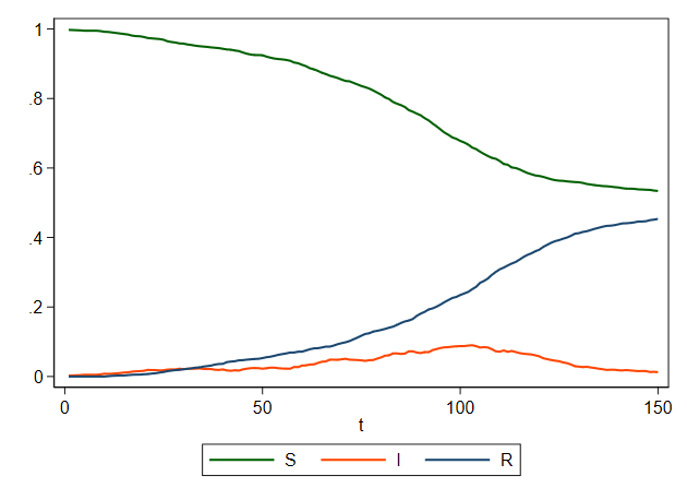
    Similarly, we can study the potential impact of policies encouraging
    social distancing or the wearing of masks by changing the
    transmissibility

. mata:
------------------------------------------------- mata (type end to exit) -----
: model.pr_loss(0)


: model.tdim(150)


: model.transmissibility(0.03)


: model.run()
----+--- 1 ---+--- 2 ---+--- 3 ---+--- 4 ---+--- 5
..................................................        50
..................................................       100
..................................................       150


: model.export_sir()


: end
-------------------------------------------------------------------------------


. 
. twoway line S I R t,  name(anc2, replace)          ///
>    ylabel(,angle(0)) legend(rows(1)) lwidth(*1.5 ..) 


. drop _all

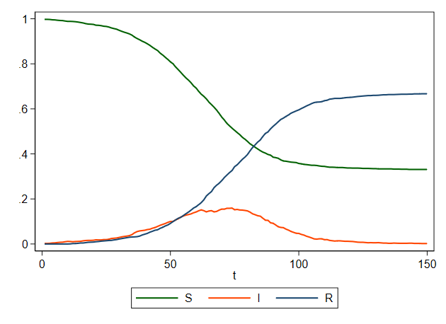
    or the potential impact of a lockdown, which would influence the number
    of people someone is in contact with

. mata:
------------------------------------------------- mata (type end to exit) -----
: model.transmissibility(0.045)


: model.mcontacts(3)


: model.run()
----+--- 1 ---+--- 2 ---+--- 3 ---+--- 4 ---+--- 5
..................................................        50
..................................................       100
..................................................       150


: model.export_sir()


: end
-------------------------------------------------------------------------------


. 
. twoway line S I R t,  name(anc3, replace)          ///
>    ylabel(,angle(0)) legend(rows(1)) lwidth(*1.5 ..) 


. drop _all

 
 
-------------------------------------------------------------------------------

 index 

-------------------------------------------------------------------------------

-------------------------------------------------------------------------------
ancillary
-------------------------------------------------------------------------------


                            Quantifying uncertainty


    ABMs are simulations, so the outcome could easily differ from run to run


    One could display the outcome from multiple runs


        Either because this gives a more complete description of an ABM


        or because this variation is interesting in and of itself

. set seed 123456789


. clear mata


. drop _all


. run sir_main.do


. 
. mata:
------------------------------------------------- mata (type end to exit) -----
: 
: model = sir()


: model.N(2000)


: model.tdim(150)


: model.outbreak(5)


: model.mcontacts(4)


: model.transmissibility(0.045)


: model.mindur(10)


: model.meandur(14)


: model.pr_loss(0)


: 
: base = "t", "S", "I", "R"


: for(i=1; i<=10; i++){
>     model.run()
>     names = J(1,4,"")
>     for(j=1; j<=4; j++) {
>         names[j] = base[j] + strofreal(i)
>     }
>     model.export_sir(names)
> }
----+--- 1 ---+--- 2 ---+--- 3 ---+--- 4 ---+--- 5
..................................................        50
..................................................       100
..................................................       150
----+--- 1 ---+--- 2 ---+--- 3 ---+--- 4 ---+--- 5
..................................................        50
..................................................       100
..................................................       150
----+--- 1 ---+--- 2 ---+--- 3 ---+--- 4 ---+--- 5
..................................................        50
..................................................       100
..................................................       150
----+--- 1 ---+--- 2 ---+--- 3 ---+--- 4 ---+--- 5
..................................................        50
..................................................       100
..................................................       150
----+--- 1 ---+--- 2 ---+--- 3 ---+--- 4 ---+--- 5
..................................................        50
..................................................       100
..................................................       150
----+--- 1 ---+--- 2 ---+--- 3 ---+--- 4 ---+--- 5
..................................................        50
..................................................       100
..................................................       150
----+--- 1 ---+--- 2 ---+--- 3 ---+--- 4 ---+--- 5
..................................................        50
..................................................       100
..................................................       150
----+--- 1 ---+--- 2 ---+--- 3 ---+--- 4 ---+--- 5
..................................................        50
..................................................       100
..................................................       150
----+--- 1 ---+--- 2 ---+--- 3 ---+--- 4 ---+--- 5
..................................................        50
..................................................       100
..................................................       150
----+--- 1 ---+--- 2 ---+--- 3 ---+--- 4 ---+--- 5
..................................................        50
..................................................       100
..................................................       150


: end
-------------------------------------------------------------------------------


. 
. twoway line S* t1, lcolor(green ..)            || ///
>        line I* t1 , lcolor(orange ..)          || ///
>        line R* t1, lcolor(blue ..)                ///
>        legend(order(1 "S" 11 "I" 21 "R") cols(3)) ///
>        ylab(,angle(0)) name(anc4, replace)

 
 
-------------------------------------------------------------------------------

 index 

-------------------------------------------------------------------------------

-------------------------------------------------------------------------------
ancillary
-------------------------------------------------------------------------------


                                Other scenarios


    We can try to quantify the impact of reducing the number of long distance
    by comparing the following models:

. clear mata


. set seed 28863


. run nw_main.do


. mata:
------------------------------------------------- mata (type end to exit) -----
: model = sir_nw()


: model.N(2000)


: model.tdim(150)


: model.outbreak(10)


: model.degree(10)


: model.pr_long(.2)


: model.transmissibility(.018)


: model.mindur(10)


: model.meandur(14)


: model.pr_loss(0.00)


: model.run()
----+--- 1 ---+--- 2 ---+--- 3 ---+--- 4 ---+--- 5
..................................................        50
..................................................       100
..................................................       150


: model.export_sir()


: end
-------------------------------------------------------------------------------


. 
. twoway line S I R t,  name(sir3, replace)          ///
>    ylabel(,angle(0)) legend(rows(1)) lwidth(*1.5 ..) 


. drop _all


. 
. mata:
------------------------------------------------- mata (type end to exit) -----
: model.pr_long(.05)


: model.run()
----+--- 1 ---+--- 2 ---+--- 3 ---+--- 4 ---+--- 5
..................................................        50
..................................................       100
..................................................       150


: model.export_sir()


: end
-------------------------------------------------------------------------------


. 
. twoway line S I R t,  name(sir4, replace)          ///
>    ylabel(,angle(0)) legend(rows(1)) lwidth(*1.5 ..) 


. 
. drop _all

 
 
-------------------------------------------------------------------------------

 index 

-------------------------------------------------------------------------------

-------------------------------------------------------------------------------
digression
-------------------------------------------------------------------------------


                                     Class


    We have a population of agents to keep track of


    We need to repeatedly apply rules to them


    Applying rules can be done by a function, but that function needs access
    to settings and the population.


    This is a good case for a class.


    A class can be thought of as a tray with named slots for functions and
    data


    The functions are local to the class


    Each function has access to all material stored in the class


 

. clear mata


. 
. mata:
------------------------------------------------- mata (type end to exit) -----
: 
: class arithmatic {
> 
>     real scalar a
>     real scalar b
>     
>     real scalar sum()
>     real scalar prod()
>     void input()
>     void run()
> }


: 
: void arithmatic::input(real scalar aval, real scalar bval)
> {
>     a = aval
>     b = bval
> }


: 
: real scalar arithmatic::sum()
> {
>     return(a + b)
> }


: 
: real scalar arithmatic::prod()
> {
>     return(a * b)
> }


: 
: void arithmatic::run()
> {
>     sum()
>     prod()
> }


: 
: // how the user interacts with this program
: math = arithmatic()


: math.input(2,4)


: math.run()
  6
  8


: end
-------------------------------------------------------------------------------

 
 
-------------------------------------------------------------------------------

<< index 

-------------------------------------------------------------------------------

-------------------------------------------------------------------------------
ancillary
-------------------------------------------------------------------------------


          Example of an ABM on a grid: Schelling's segregation model


    In this model there are blue and red agents, that live in cells on a
    square grid.  Each cell can contain only one agent, but not all cells are
    occupied. An agent is happy if the proportion of agents of the same
    colour in her neighbourhood is above a certain cut-off value. If she is
    unhappy she will move to the nearest available cell that does satisfy her
    needs.


    The point of this simulation that even with a low cut-off value, like
    30%, you will get fairly seggregated neighbourhoods.

. clear mata


. drop _all


. set seed 1234567


. 
. run schelling_main.mata


. 
. mata:
------------------------------------------------- mata (type end to exit) -----
: model = schelling()


: model.rdim(10)


: model.cdim(10)


: model.tdim(5)


: model.nred(45)


: model.nblue(45)


: model.limit(.3)


: model.run()


: model.summtable()


Average proportion of neighbours with same color and average proportion of
happy agents


-----------------------------------
 Iteration   prop same  prop happy 
-----------------------------------
         0        .543        .867 
         1        .688        .944 
         2        .725        .978 
         3        .738        .978 
         4        .768        .989 
         5        .768        .989 
-----------------------------------


: model.extract(("r","c","t", "id", "red", "happy"))


: end
-------------------------------------------------------------------------------


. 
. replace r = -r
(540 real changes made)


. 
. forvalues t = 0/5 {
  2.     twoway scatter r c if red == 0 & t == `t' & happy == 1, ///
>            msymbol(O) mcolor(blue) msize(*2)                ///
>            mlabel(id) mlabpos(0)                         || ///
>            scatter r c if red == 1 & t == `t' & happy == 1, ///
>            msymbol(O) mcolor(red) msize(*2)                 ///
>            mlabel(id) mlabpos(0)                         || ///
>            scatter r c if red == 0 & t == `t' & happy == 0, ///
>            msymbol(Oh) mcolor(blue) msize(*2)               ///
>            mlabel(id) mlabpos(0)                         || ///
>            scatter r c if red == 1 & t == `t' & happy == 0, ///
>            msymbol(Oh) mcolor(red) msize(*2)                ///
>            mlabel(id) mlabpos(0)                            ///
>            yscale(off range(-10.5 -.5))                     ///
>            xscale(off  range(.5 10.5))                      ///
>            ylab(none) xlab(none)                            ///
>            plotregion(margin(zero))                         ///
>            aspect(1)                                        ///
>            xline(.5(1)9.5)                                  ///
>            yline(-.5(-1)-9.5)                               ///
>            legend(off)                                      ///
>            name(gr`t', replace) title(Iteration `t')
  3. }

 
 
-------------------------------------------------------------------------------

 index 

-------------------------------------------------------------------------------