-------------------------------------------------------------------------------
Example presentation: stdtable, a package to standardize tables --
standardizing cross-tabulations
-------------------------------------------------------------------------------


                    The influence of marginal distributions


    Consider the example below


    It shows the race of the husband and the race of the wife for couples
    living in the USA that got married between 2010 and 2017


    The races are very unequaly distributed in the USA


    We can control for one marginal distribution by computing row or collumn
    percentages.
. use homogamy, clear
(American Community Survey 2008-2017)


. tab racem racef [fw=freq] if marcoh == 2010, row nofreq


     race, |                       race, wife
   husband |     white   hispanic      black     native      asian |     Total
-----------+-------------------------------------------------------+----------
     white |     89.55       5.16       0.76       0.38       2.56 |    100.00
  hispanic |     18.25      77.54       1.19       0.27       1.55 |    100.00
     black |     13.02       5.46      77.49       0.24       1.40 |    100.00
    native |     46.04       6.90       1.44      41.55       2.19 |    100.00
     asian |      9.83       2.60       0.42       0.07      85.64 |    100.00
     other |     46.29      11.58       5.20       0.68       7.83 |    100.00
-----------+-------------------------------------------------------+----------
     Total |     64.27      17.56       8.14       0.55       7.36 |    100.00


     race, | race, wife
   husband |     other |     Total
-----------+-----------+----------
     white |      1.60 |    100.00
  hispanic |      1.20 |    100.00
     black |      2.39 |    100.00
    native |      1.89 |    100.00
     asian |      1.43 |    100.00
     other |     28.42 |    100.00
-----------+-----------+----------
     Total |      2.12 |    100.00
    We see racial homogamy: people tend to marry someone of the same race


    However, several things are hard to see in this table:


        Are whites really the most closed group or is there a substantial
        "colorblind" group of whites that accidentally married another white
        because that is the largest group?


        Are Native Americans really so much less homogamous or are we seeing
        an artifact caused by the small number of native american women
        (0.6%)?


        If native Americans were mixing around randomly, then we would expect
        much less native american males marrying native american females.
        Apperently native American men still prefer native American women but
        because there are so many other women around he will still have a
        good chance of eventually marrying another women.


        Is there symetery in this table, e.g. are hispanic males as likely to
        marry a white female as hispanic females are to marry white males?


        It does not seem to be the case from this table, but 5% from all
        white males could be similar to 18% from all hispanic males.


    There is something mechanical about the influence of the margins, and it
    is common (in sociology) to want to look at the pattern in the table nett
    of this influence of the marginal distributions.


    We could do this by looking at >> odds ratios, but here I want to show an
    alternative.


-------------------------------------------------------------------------------
index >>
-------------------------------------------------------------------------------
-------------------------------------------------------------------------------
Example presentation: stdtable, a package to standardize tables --
standardizing cross-tabulations
-------------------------------------------------------------------------------


                             Standardizing tables


    When we do a chi squared test for cross-tabulations we compare observed
    cell counts with predicted cell counts


    For these predicted cell counts we assume that the margins remain as
    observed, but otherwise there is no association between the variables
    (the odds ratios are all 1).


    In the table of predicted cell counts the only pattern is due to the
    margins.
. tab racem racef [fw=freq] if marcoh==2010, exp


+--------------------+
| Key                |
|--------------------|
|     frequency      |
| expected frequency |
+--------------------+


     race, |                       race, wife
   husband |     white   hispanic      black     native      asian |     Total
-----------+-------------------------------------------------------+----------
     white |31,956,989  1,842,451    270,679    134,486    911,938 |35,687,890
           |22935235.6  6267911.2  2904780.0  197,859.6  2625311.4 |35687890.0
-----------+-------------------------------------------------------+----------
  hispanic | 1,716,537  7,292,537    111,903     25,163    145,556 | 9,404,856
           | 6044139.6  1651787.3  765,498.8   52,142.1  691,850.2 | 9404856.0
-----------+-------------------------------------------------------+----------
     black |   674,410    282,817  4,014,816     12,534     72,745 | 5,181,272
           | 3329804.4  909,993.6  421,724.4   28,725.8  381,150.4 | 5181272.0
-----------+-------------------------------------------------------+----------
    native |   136,200     20,397      4,253    122,904      6,469 |   295,799
           | 190,098.7   51,951.6   24,076.3    1,640.0   21,759.9 | 295,799.0
-----------+-------------------------------------------------------+----------
     asian |   323,750     85,783     13,922      2,216  2,820,542 | 3,293,314
           | 2116486.4  578,409.1  268,056.0   18,258.7  242,266.3 | 3293314.0
-----------+-------------------------------------------------------+----------
     other |   494,673    123,760     55,546      7,248     83,703 | 1,068,672
           | 686,794.4  187,692.3   86,983.5    5,924.9   78,614.8 | 1068672.0
-----------+-------------------------------------------------------+----------
     Total |35,302,559  9,647,745  4,471,119    304,551  4,040,953 |54,931,803
           |35302559.0  9647745.0  4471119.0  304,551.0  4040953.0 |54931803.0


     race, | race, wife
   husband |     other |     Total
-----------+-----------+----------
     white |   571,347 |35,687,890
           | 756,792.3 |35687890.0
-----------+-----------+----------
  hispanic |   113,160 | 9,404,856
           | 199,438.0 | 9404856.0
-----------+-----------+----------
     black |   123,950 | 5,181,272
           | 109,873.3 | 5181272.0
-----------+-----------+----------
    native |     5,576 |   295,799
           |   6,272.7 | 295,799.0
-----------+-----------+----------
     asian |    47,101 | 3,293,314
           |  69,837.5 | 3293314.0
-----------+-----------+----------
     other |   303,742 | 1,068,672
           |  22,662.1 | 1068672.0
-----------+-----------+----------
     Total | 1,164,876 |54,931,803
           | 1164876.0 |54931803.0
    Can't we reverse that? Keep the association (odds ratios) as observed but
    fix the margins.


    For example we could fix all margins at a 100.


    That way we can look at the proportion native American men marrying
    native American women when they weren't such a small group.


    This is what standardizing tables does (Yule 1912). This is implemented
    in the stdtable package.
. stdtable racem racef [fw=freq] if marcoh == 2010


-------------------------------------------------------------------------------
race,    |                              race, wife
husband  |    white  hispanic     black    native     asian     other     Total
---------+---------------------------------------------------------------------
   white |     67.3      8.29      2.72      4.88      4.87      11.9       100
hispanic |     8.69      78.9      2.71      2.19      1.87      5.68       100
   black |     3.05      2.74      86.8      .978      .835      5.56       100
  native |      5.7      1.82      .851      88.6      .686      2.31       100
   asian |     3.94      2.23      .809      .464      86.9      5.67       100
   other |     11.3      6.05      6.07      2.86      4.85      68.9       100
         |
   Total |      100       100       100       100       100       100       600
-------------------------------------------------------------------------------
    stdtable is thus very useful in conjunction with a chi-squared test for
    cross-tabulations:


        The chi-squared test tells you whether or not there is a pattern in
        the table on top of what is imposed by the margins.


        stdtable tells you what that pattern is.


-------------------------------------------------------------------------------
<< index >>
-------------------------------------------------------------------------------
-------------------------------------------------------------------------------
Example presentation: stdtable, a package to standardize tables --
standardizing cross-tabulations
-------------------------------------------------------------------------------


                       Displaying results from stdtable


    We can add options to make the table look better
. stdtable racem racef [fw=freq] if marcoh == 2010, ///
>          format(%5.0f)


-------------------------------------------------------------------------------
race,    |                              race, wife
husband  |    white  hispanic     black    native     asian     other     Total
---------+---------------------------------------------------------------------
   white |       67         8         3         5         5        12       100
hispanic |        9        79         3         2         2         6       100
   black |        3         3        87         1         1         6       100
  native |        6         2         1        89         1         2       100
   asian |        4         2         1         0        87         6       100
   other |       11         6         6         3         5        69       100
         |
   Total |      100       100       100       100       100       100       600
-------------------------------------------------------------------------------
We can compare across groups
. stdtable racem racef [fw=freq], by(marcoh) format(%5.0f)


--------------------------------------------------------------------------
mariage   |
cohort    |
and race, |                           race, wife
husband   |    white hispanic    black   native    asian    other    Total
----------+---------------------------------------------------------------
1950-1959 |
    white |       88        2        0        3        1        5      100
 hispanic |        3       95        0        1        0        1      100
    black |        0        0       97        0        0        2      100
   native |        3        1        1       93        0        3      100
    asian |        1        1        0        0       95        3      100
    other |        6        1        2        2        3       86      100
          |
    Total |      100      100      100      100      100      100      600
----------+---------------------------------------------------------------
1960-1969 |
    white |       86        3        0        4        2        6      100
 hispanic |        3       94        0        1        0        1      100
    black |        0        0       96        0        0        2      100
   native |        4        1        0       93        0        2      100
    asian |        1        1        0        0       95        3      100
    other |        6        1        2        2        2       86      100
          |
    Total |      100      100      100      100      100      100      600
----------+---------------------------------------------------------------
1970-1979 |
    white |       82        4        0        5        2        6      100
 hispanic |        4       92        1        1        1        2      100
    black |        1        1       95        1        1        2      100
   native |        5        1        1       91        0        2      100
    asian |        2        1        0        0       94        3      100
    other |        6        2        3        2        2       84      100
          |
    Total |      100      100      100      100      100      100      600
----------+---------------------------------------------------------------
1980-1989 |
    white |       79        5        1        5        3        7      100
 hispanic |        5       89        1        2        1        2      100
    black |        1        1       94        1        1        3      100
   native |        5        1        1       91        1        2      100
    asian |        2        1        0        0       93        4      100
    other |        8        3        3        2        3       82      100
          |
    Total |      100      100      100      100      100      100      600
----------+---------------------------------------------------------------
1990-1999 |
    white |       75        6        2        5        3        9      100
 hispanic |        6       87        2        2        1        3      100
    black |        2        1       92        1        1        3      100
   native |        6        1        1       89        0        3      100
    asian |        2        1        0        1       91        4      100
    other |        9        3        3        3        3       79      100
          |
    Total |      100      100      100      100      100      100      600
----------+---------------------------------------------------------------
2000-2009 |
    white |       70        8        2        5        4       10      100
 hispanic |        7       82        2        3        1        5      100
    black |        2        2       89        1        1        4      100
   native |        6        2        1       88        1        3      100
    asian |        3        2        1        1       88        5      100
    other |       10        5        5        2        5       73      100
          |
    Total |      100      100      100      100      100      100      600
----------+---------------------------------------------------------------
2010-2017 |
    white |       67        8        3        5        5       12      100
 hispanic |        9       79        3        2        2        6      100
    black |        3        3       87        1        1        6      100
   native |        6        2        1       89        1        2      100
    asian |        4        2        1        0       87        6      100
    other |       11        6        6        3        5       69      100
          |
    Total |      100      100      100      100      100      100      600
--------------------------------------------------------------------------
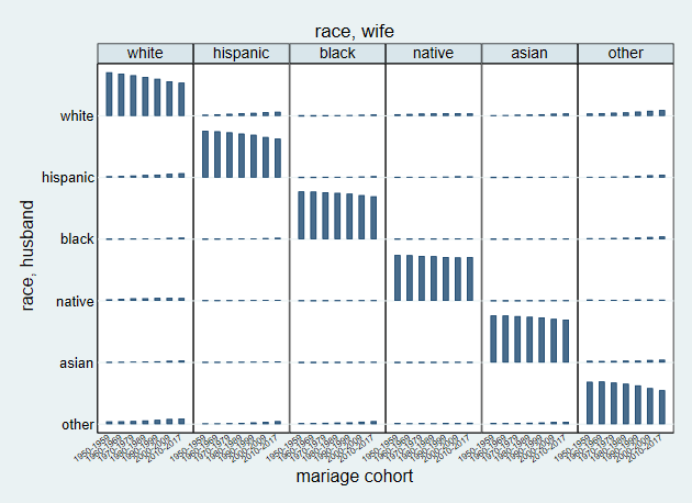
    Alternatively we can replace the data in memory with standardized counts
    and use those to create a graph
. qui stdtable racem racef [fw=freq],          ///
>     by(marcoh) replace


.
. tabplot racem marcoh [iw=std],               ///
>     by(racef, compact note("") cols(6)       ///
>        t1title("race, wife"))                ///
>     xlab( 1(1)7, angle(35) labsize(vsmall) )
-------------------------------------------------------------------------------
<< index >>
-------------------------------------------------------------------------------
-------------------------------------------------------------------------------
Example presentation: stdtable, a package to standardize tables -- Estimation
-------------------------------------------------------------------------------


                        Iterative Proportional fitting


    The idea to change the margins to be all 100, but otherwise leave
    everything as much as possible the same.


    We know how to do that for just row totals:


        divide all cells by its rowtotal and multiply by 100
. use homogamy, clear
(American Community Survey 2008-2017)


. tab racem racef [fw=freq] if marcoh == 2010, matcell(data)


     race, |                       race, wife
   husband |     white   hispanic      black     native      asian |     Total
-----------+-------------------------------------------------------+----------
     white |31,956,989  1,842,451    270,679    134,486    911,938 |35,687,890
  hispanic | 1,716,537  7,292,537    111,903     25,163    145,556 | 9,404,856
     black |   674,410    282,817  4,014,816     12,534     72,745 | 5,181,272
    native |   136,200     20,397      4,253    122,904      6,469 |   295,799
     asian |   323,750     85,783     13,922      2,216  2,820,542 | 3,293,314
     other |   494,673    123,760     55,546      7,248     83,703 | 1,068,672
-----------+-------------------------------------------------------+----------
     Total |35,302,559  9,647,745  4,471,119    304,551  4,040,953 |54,931,803


     race, | race, wife
   husband |     other |     Total
-----------+-----------+----------
     white |   571,347 |35,687,890
  hispanic |   113,160 | 9,404,856
     black |   123,950 | 5,181,272
    native |     5,576 |   295,799
     asian |    47,101 | 3,293,314
     other |   303,742 | 1,068,672
-----------+-----------+----------
     Total | 1,164,876 |54,931,803


.
. mata
------------------------------------------------- mata (type end to exit) -----
: data = st_matrix("data")


:
: muhat = data


:
: muhat = muhat:/rowsum(muhat):*100


: end
-------------------------------------------------------------------------------
We could do the same with the column totals
. mata
------------------------------------------------- mata (type end to exit) -----
: muhat = muhat:/colsum(muhat):*100


: colsum(muhat)
         1     2     3     4     5     6
    +-------------------------------------+
  1 |  100   100   100   100   100   100  |
    +-------------------------------------+


: rowsum(muhat)
                 1
    +---------------+
  1 |  53.49494192  |
  2 |  85.94806215  |
  3 |   108.846317  |
  4 |  132.1110102  |
  5 |  95.96333662  |
  6 |  123.6363322  |
    +---------------+


: end
-------------------------------------------------------------------------------
    This is close, but not quite.


    What happens when we repeat that a couple of times
. mata
------------------------------------------------- mata (type end to exit) -----
: muhat = muhat:/rowsum(muhat):*100


: muhat = muhat:/colsum(muhat):*100


:
: muhat = muhat:/rowsum(muhat):*100


: muhat = muhat:/colsum(muhat):*100


:
: muhat = muhat:/rowsum(muhat):*100


: muhat = muhat:/colsum(muhat):*100


:
: muhat = muhat:/rowsum(muhat):*100


: muhat = muhat:/colsum(muhat):*100


: colsum(muhat)
         1     2     3     4     5     6
    +-------------------------------------+
  1 |  100   100   100   100   100   100  |
    +-------------------------------------+


: rowsum(muhat)
                 1
    +---------------+
  1 |  98.64518228  |
  2 |  97.08558589  |
  3 |  101.6611192  |
  4 |  106.2503037  |
  5 |  97.30651588  |
  6 |  99.05129309  |
    +---------------+


: end
-------------------------------------------------------------------------------
    Again, better and we can imagine that with some extra iterations we would
    get where we want to be.


    This is iterative proportional fitting (Kruithof 1937; Deming and Stephan
    1940)


-------------------------------------------------------------------------------
<< index >>
-------------------------------------------------------------------------------
-------------------------------------------------------------------------------
How to create a smcl presentation -- creating the presentation
-------------------------------------------------------------------------------


                                Getting started


    I start with creating a folder for my presentation, with three
    sub-folders:


        source
        presentation
        handout


    I then start brainstorming about what I want to do in my presentation.


    I typically do this in a text file in the source directory, that will
    later become a .do file, so I put the text in comments


    Here is the .do file for the example presentation
// -------- A section standardizing cross-tabulations

// illustrate the impact of the marginal distribution in cross-tabulations with
// an example

// a digression on odds ratios

// Show how the chi-squared test deals with marginal distributions

// Standardizing tables as the reverse of chi-squared test

// -------- A section on Iterative proportional fitting

// use Mata to repeatedly make all row totals a 100, and all column totals 100

// a appendix showing that not all tables can be standardized
Next step is to create the examples
// -------- A section standardizing cross-tabulations

// illustrate the impact of the marginal distribution in cross-tabulations with
// an example

use homogamy, clear
tab racem racef [fw=freq] if marcoh == 2010, row nofreq

// a digression on odds ratios
tab racem racef [fw=freq] if marcoh == 2010
di 122904 / 136200
di 134486 / 31956989
di (122904 / 136200)/(134486 / 31956989)

// Show how the chi-squared test deals with marginal distributions

tab racem racef [fw=freq] if marcoh==2010, exp

// Standardizing tables as the reverse of chi-squared test

stdtable racem racef [fw=freq] if marcoh == 2010

// show how to make the table look better, compare groups, and turn it into a graph

stdtable racem racef [fw=freq] if marcoh == 2010, ///
         format(%5.0f)

stdtable racem racef [fw=freq], by(marcoh) format(%5.0f)

qui stdtable racem racef [fw=freq],          ///
    by(marcoh) replace

tabplot racem marcoh [iw=std],               ///
    by(racef, compact note("") cols(6)       ///
	   t1title("race, wife"))                ///
    xlab( 1(1)7, angle(35) labsize(vsmall) )

// -------- A section on Iterative proportional fitting

// use Mata to repeatedly make all row totals a 100, and all column totals 100

use homogamy, clear
tab racem racef [fw=freq] if marcoh == 2010, matcell(data)

mata
data = st_matrix("data")

muhat = data

muhat = muhat:/rowsum(muhat):*100
end

mata
muhat = muhat:/colsum(muhat):*100
colsum(muhat)
rowsum(muhat)
end

mata
muhat = muhat:/rowsum(muhat):*100
muhat = muhat:/colsum(muhat):*100

muhat = muhat:/rowsum(muhat):*100
muhat = muhat:/colsum(muhat):*100

muhat = muhat:/rowsum(muhat):*100
muhat = muhat:/colsum(muhat):*100

muhat = muhat:/rowsum(muhat):*100
muhat = muhat:/colsum(muhat):*100
colsum(muhat)
rowsum(muhat)
end

// a appendix showing that not all tables can be standardized

/*
        0 0 2
        1 5 2
        8 7 0
*/
    Next step is to Indicate when a slide begins with //slide and ends with
    //endslide


    With the //title one specifies the title of the slide


    Examples are indicated by //ex and //endex


    Indicate any datasets or other files that the presentation needs with
    //file filename


    Sections are indicated by //section section_name


    This is what we get:
//section standardizing cross-tabulations

//slide ------------------------------------------------------------------------
//title The influence of marginal distributions

//ex
use homogamy, clear
tab racem racef [fw=freq] if marcoh == 2010, row nofreq
//endex

//endslide ---------------------------------------------------------------------

//slide ------------------------------------------------------------------------
//title Odds ratios
//ex
tab racem racef [fw=freq] if marcoh == 2010
di 122904 / 136200
di 134486 / 31956989
di (122904 / 136200)/(134486 / 31956989)
//endex
//endslide ---------------------------------------------------------------------


//slide ------------------------------------------------------------------------
//title Standardizing tables
//ex
tab racem racef [fw=freq] if marcoh==2010, exp
//endex

//ex
stdtable racem racef [fw=freq] if marcoh == 2010
//endex
//endslide ---------------------------------------------------------------------

//slide ------------------------------------------------------------------------
//title Displaying results from stdtable

//ex
stdtable racem racef [fw=freq] if marcoh == 2010, ///
         format(%5.0f)
//endex

//ex
stdtable racem racef [fw=freq], by(marcoh) format(%5.0f)
//endex

//ex
qui stdtable racem racef [fw=freq],          ///
    by(marcoh) replace

tabplot racem marcoh [iw=std],               ///
    by(racef, compact note("") cols(6)       ///
	   t1title("race, wife"))                ///
    xlab( 1(1)7, angle(35) labsize(vsmall) )
//endex
//endslide ---------------------------------------------------------------------

//section Estimation
//slide ------------------------------------------------------------------------
//title Iterative Proportional fitting

//ex
use homogamy, clear
tab racem racef [fw=freq] if marcoh == 2010, matcell(data)

mata
data = st_matrix("data")

muhat = data

muhat = muhat:/rowsum(muhat):*100
end
//endex

//ex
mata
muhat = muhat:/colsum(muhat):*100
colsum(muhat)
rowsum(muhat)
end
//endex

//ex
mata
muhat = muhat:/rowsum(muhat):*100
muhat = muhat:/colsum(muhat):*100

muhat = muhat:/rowsum(muhat):*100
muhat = muhat:/colsum(muhat):*100

muhat = muhat:/rowsum(muhat):*100
muhat = muhat:/colsum(muhat):*100

muhat = muhat:/rowsum(muhat):*100
muhat = muhat:/colsum(muhat):*100
colsum(muhat)
rowsum(muhat)
end
//endex
//endslide ---------------------------------------------------------------------

//slide ------------------------------------------------------------------------
//title Can all tables be standardized?

/*
        0 0 2
        1 5 2
        8 7 0
*/
//endslide ---------------------------------------------------------------------
This is already a sourcefile we can use for smclpres
. smclpres using stdtable\source\stdtable03.do , replace dir(stdtable/presentat
> ion)
to view the presentation:
first change the directory to where the presentation is stored:
cd "D:\Mijn
documenten\projecten\stata\sug\london19\buis_smclpres\presentation\stdtable\pre
> sentation"
Then type:
view stdtable03.smcl


. cd stdtable/presentation
D:\Mijn documenten\projecten\stata\sug\london19\buis_smclpres\presentation\stdt
> able\presentation


. dir
  <dir>   9/03/19 10:06  .
  <dir>   9/03/19 10:06  ..
   6.3k   8/06/19 11:07  homogamy.dta
   0.5k   9/03/19 10:06  slide1.smcl
   0.1k   9/03/19 10:06  slide1ex1.do
   0.5k   9/03/19 10:06  slide2.smcl
   0.1k   9/03/19 10:06  slide2ex1.do
   0.6k   9/03/19 10:06  slide3.smcl
   0.0k   9/03/19 10:06  slide3ex1.do
   0.0k   9/03/19 10:06  slide3ex2.do
   1.1k   9/03/19 10:06  slide4.smcl
   0.1k   9/03/19 10:06  slide4ex1.do
   0.1k   9/03/19 10:06  slide4ex2.do
   0.3k   9/03/19 10:06  slide4ex3.do
   1.4k   9/03/19 10:06  slide5.smcl
   0.2k   9/03/19 10:06  slide5ex1.do
   0.1k   9/03/19 10:06  slide5ex2.do
   0.3k   9/03/19 10:06  slide5ex3.do
   0.2k   9/03/19 10:06  slide6.smcl
   0.8k   9/03/19 10:03  slide7.smcl
   0.3k   9/03/19 10:06  stdtable03.smcl
   0.3k   9/03/19  9:54  stdtable04.smcl
   0.4k   8/08/19 11:46  stdtable05.smcl
   0.9k   9/03/19  9:58  stdtable06.smcl
   0.9k   8/08/19 11:46  stdtable07.smcl
   0.9k   9/03/19 10:03  stdtable08.smcl


. cd ../..
D:\Mijn documenten\projecten\stata\sug\london19\buis_smclpres\presentation
-------------------------------------------------------------------------------
<< index >>
-------------------------------------------------------------------------------
-------------------------------------------------------------------------------
How to create a smcl presentation -- creating the presentation
-------------------------------------------------------------------------------


                                  Adding text


    You can add a text block by starting a line with /*txt and ending it with
    txt*/


    The text will be formatted using SMCL, which is documented in help smcl


    The most important directives are:


        {pstd} starts a standard paragraph


        {pmore} starts an indented paragraph


        {p_end} ends a paragraph


        {help cmd_name} adds a link to the helpfile of cmd_name.


    The sourcefile after including text looks like this:
//file homogamy.dta

//section standardizing cross-tabulations

//slide ------------------------------------------------------------------------
//title The influence of marginal distributions

/*txt
{pstd}
Consider the example below

{pstd}
It shows the race of the husband and the race of the wife for couples living in
the USA that got married between 2010 and 2017

{pstd}
The races are very unequaly distributed in the USA

{pstd}
We can control for one marginal distribution by computing row or collumn
percentages.
txt*/

//ex
use homogamy, clear
tab racem racef [fw=freq] if marcoh == 2010, row nofreq
//endex

/*txt
{pstd}
We see racial homogamy: people tend to marry someone of the same race

{pstd}
However, several things are hard to see in this table:

{pmore}
{cmd:Are whites really the most closed group} or is there a substantial
"colorblind" group of whites that accidentally married another white because that
is the largest group?

{pmore}
{cmd:Are Native Americans really so much less homogamous} or are we seeing an
artifact caused by the small number of native american women (0.6%)?

{pmore}
If native Americans were mixing around randomly, then we would expect much less
native american males marrying native american females. Apperently native
American men still prefer native American women but because there are so many
other women around he will still have a good chance of eventually marrying another
women.

{pmore}
{cmd:Is there symetery in this table}, e.g. are hispanic males as likely to marry a
white female as hispanic females are to marry white males?

{pmore}
It does not seem to be the case from this table, but 5% from all white males
could be similar to 18% from all hispanic males.

{pstd}
There is something mechanical about the influence of the margins, and it is
common (in sociology) to want to look at the pattern in the table nett of this
influence of the marginal distributions.

{pstd}
We could do this by looking at odds ratios , but here I want to show an alternative.
txt*/

//endslide ---------------------------------------------------------------------

//slide ------------------------------------------------------------------------
//title Odds ratios

/*txt
{pstd}
The odds is the number of "successes" per "failure"

{pstd}
The odds ratio is a ratio of odds, and this measure of association is indpendent
of the marginal distributions
txt*/

//ex
tab racem racef [fw=freq] if marcoh == 2010
di 122904 / 136200
di 134486 / 31956989
di (122904 / 136200)/(134486 / 31956989)
//endex

/*txt
{pstd}
The odds that a native ameriance man marries a native american women and not a
white women is 0.9.

{pmore}
The odds that a white man marries a native american women and not a white women
is 0.004.

{pstd}
The odds of marrying a native american women compared to a white women is 214
times larger for native American man than for white man.

txt*/
//endslide  --------------------------------------------------------------------


//slide ------------------------------------------------------------------------
//title Standardizing tables

/*txt
{pstd}
When we do a chi squared test for cross-tabulations we compare observed cell counts
with predicted cell counts

{pstd}
For these predicted cell counts we assume that the margins remain as observed,
but otherwise there is no association between the variables (the odds ratios are
all 1).

{pstd}
In the table of predicted cell counts the only pattern is due to the margins.
txt*/

//ex
tab racem racef [fw=freq] if marcoh==2010, exp
//endex

/*txt
{pstd}
Can't we reverse that? Keep the association (odds ratios) as observed but fix
the margins.

{pstd}
For example we could fix all margins at a 100.

{pstd}
That way we can look at the proportion native American men marrying native American
women when they weren't such a small group.

{pstd}
This is what standardizing tables does (Yule 1912). This is implemented in the
{helpb stdtable} package.
txt*/

//ex
stdtable racem racef [fw=freq] if marcoh == 2010
//endex

/*txt
{pstd}
{cmd:stdtable} is thus very useful in conjunction with a chi-squared test for
cross-tabulations:

{pmore}
The chi-squared test tells you whether or not there is a pattern in the table
that is significantly different from independence

{pmore}
{cmd:stdtable} tells you what that pattern is.
txt*/
//endslide ---------------------------------------------------------------------

//slide ------------------------------------------------------------------------
//title Displaying results from stdtable

/*txt
{pstd}
We can add options to make the table look better
txt*/

//ex
stdtable racem racef [fw=freq] if marcoh == 2010, ///
         format(%5.0f)
//endex


/*txt
We can compare across groups
txt*/

//ex
stdtable racem racef [fw=freq], by(marcoh) format(%5.0f)
//endex

/*txt
{pstd}
Alternatively we can replace the data in memory with standardized counts and
use those to create a graph
txt*/

//ex
qui stdtable racem racef [fw=freq],          ///
    by(marcoh) replace

tabplot racem marcoh [iw=std],               ///
    by(racef, compact note("") cols(6)       ///
	   t1title("race, wife"))                ///
    xlab( 1(1)7, angle(35) labsize(vsmall) )
//endex

//endslide ---------------------------------------------------------------------

//section Estimation
//slide ------------------------------------------------------------------------
//title Iterative Proportional fitting

/*txt
{pstd}
The idea to change the margins to be all 100, but otherwise leave everything as
much as possible the same.

{pstd}
We know how to do that for just row totals:

{pmore}
divide all cells by its rowtotal and multiply by 100
txt*/

//ex
use homogamy, clear
tab racem racef [fw=freq] if marcoh == 2010, matcell(data)

mata
data = st_matrix("data")

muhat = data

muhat = muhat:/rowsum(muhat):*100
end
//endex

/*txt
{pstd}
We could do the same with the column totals
txt*/

//ex
mata
muhat = muhat:/colsum(muhat):*100
colsum(muhat)
rowsum(muhat)
end
//endex

/*txt
{pstd}
This is close, but not quite.

{pstd}
What happens when we repeat that a couple of times
txt*/

//ex
mata
muhat = muhat:/rowsum(muhat):*100
muhat = muhat:/colsum(muhat):*100

muhat = muhat:/rowsum(muhat):*100
muhat = muhat:/colsum(muhat):*100

muhat = muhat:/rowsum(muhat):*100
muhat = muhat:/colsum(muhat):*100

muhat = muhat:/rowsum(muhat):*100
muhat = muhat:/colsum(muhat):*100
colsum(muhat)
rowsum(muhat)
end
//endex

/*txt
{pstd}
Again, better and we can imagine that with some extra iterations we would get
where we want to be.

{pstd}
This is iterative proportional fitting (Kruithof 1937; Deming and Stephan 1940)
txt*/
//endslide ---------------------------------------------------------------------

//slide ------------------------------------------------------------------------
//title Can all tables be standardized?

/*txt
{pstd}Consider the following table{p_end}

        0 0 2
        1 5 2
        8 7 0

{pstd}In order to make the first row total 100, the top right cell {it:must} be
100{p_end}

{pstd}In order to make the last column total 100, the top right cell {it:cannot}
be 100{p_end}

{pstd}This is an example of a table that cannot be standardized, and the algorithm
will not converge.
txt*/
//endslide ---------------------------------------------------------------------
. smclpres using stdtable\source\stdtable04.do , replace dir(stdtable/presentat
> ion)
to view the presentation:
first change the directory to where the presentation is stored:
cd "D:\Mijn
documenten\projecten\stata\sug\london19\buis_smclpres\presentation\stdtable\pre
> sentation"
Then type:
view stdtable04.smcl
-------------------------------------------------------------------------------
<< index >>
-------------------------------------------------------------------------------
-------------------------------------------------------------------------------
How to create a smcl presentation -- creating the presentation
-------------------------------------------------------------------------------


                           Different kinds of slides


    The normal slides (what we have used thus far) represent the main linear
    flow of the presentation.


    We can also add digression slides. The arrows at the bottom of a slide
    will skip it, but you must add a link to it in a text block on the
    previous regular slide.


    So during the presentation, the presenter can easily decide whether or
    not to skip the digression slide.


        You specify the digression slide using //digr and //enddigr


        You specify the where the link will appear in the previous slide
        using /*digr*/


        You specify the label used for the link using //label


    Alternatively we can add a ancillary slide, which can only be accessed
    from the index slide


    This type of slide serves the purpose of an appendix.


        You specify the ancillary slide using //anc and //endanc


    The sourcefile after including a digression and an ancillary slide looks
    like this:
//file homogamy.dta

//section standardizing cross-tabulations

//slide ------------------------------------------------------------------------
//title The influence of marginal distributions

/*txt
{pstd}
Consider the example below

{pstd}
It shows the race of the husband and the race of the wife for couples living in
the USA that got married between 2010 and 2017

{pstd}
The races are very unequaly distributed in the USA

{pstd}
We can control for one marginal distribution by computing row or collumn
percentages.
txt*/

//ex
use homogamy, clear
tab racem racef [fw=freq] if marcoh == 2010, row nofreq
//endex

/*txt
{pstd}
We see racial homogamy: people tend to marry someone of the same race

{pstd}
However, several things are hard to see in this table:

{pmore}
{cmd:Are whites really the most closed group} or is there a substantial
"colorblind" group of whites that accidentally married another white because that
is the largest group?

{pmore}
{cmd:Are Native Americans really so much less homogamous} or are we seeing an
artifact caused by the small number of native american women (0.6%)?

{pmore}
If native Americans were mixing around randomly, then we would expect much less
native american males marrying native american females. Apperently native
American men still prefer native American women but because there are so many
other women around he will still have a good chance of eventually marrying another
women.

{pmore}
{cmd:Is there symetery in this table}, e.g. are hispanic males as likely to marry a
white female as hispanic females are to marry white males?

{pmore}
It does not seem to be the case from this table, but 5% from all white males
could be similar to 18% from all hispanic males.

{pstd}
There is something mechanical about the influence of the margins, and it is
common (in sociology) to want to look at the pattern in the table nett of this
influence of the marginal distributions.

{pstd}
We could do this by looking at /*digr*/ , but here I want to show an alternative.
txt*/

//endslide ---------------------------------------------------------------------

//digr -------------------------------------------------------------------------
//title Odds ratios
//label odds ratios

/*txt
{pstd}
The odds is the number of "successes" per "failure"

{pstd}
The odds ratio is a ratio of odds, and this measure of association is indpendent
of the marginal distributions
txt*/

//ex
tab racem racef [fw=freq] if marcoh == 2010
di 122904 / 136200
di 134486 / 31956989
di (122904 / 136200)/(134486 / 31956989)
//endex

/*txt
{pstd}
The odds that a native ameriance man marries a native american women and not a
white women is 0.9.

{pmore}
The odds that a white man marries a native american women and not a white women
is 0.004.

{pstd}
The odds of marrying a native american women compared to a white women is 214
times larger for native American man than for white man.

txt*/
//enddigr ----------------------------------------------------------------------


//slide ------------------------------------------------------------------------
//title Standardizing tables

/*txt
{pstd}
When we do a chi squared test for cross-tabulations we compare observed cell counts
with predicted cell counts

{pstd}
For these predicted cell counts we assume that the margins remain as observed,
but otherwise there is no association between the variables (the odds ratios are
all 1).

{pstd}
In the table of predicted cell counts the only pattern is due to the margins.
txt*/

//ex
tab racem racef [fw=freq] if marcoh==2010, exp
//endex

/*txt
{pstd}
Can't we reverse that? Keep the association (odds ratios) as observed but fix
the margins.

{pstd}
For example we could fix all margins at a 100.

{pstd}
That way we can look at the proportion native American men marrying native American
women when they weren't such a small group.

{pstd}
This is what standardizing tables does (Yule 1912). This is implemented in the
{helpb stdtable} package.
txt*/

//ex
stdtable racem racef [fw=freq] if marcoh == 2010
//endex

/*txt
{pstd}
{cmd:stdtable} is thus very useful in conjunction with a chi-squared test for
cross-tabulations:

{pmore}
The chi-squared test tells you whether or not there is a pattern in the table
that is significantly different from independence

{pmore}
{cmd:stdtable} tells you what that pattern is.
txt*/
//endslide ---------------------------------------------------------------------

//slide ------------------------------------------------------------------------
//title Displaying results from stdtable

/*txt
{pstd}
We can add options to make the table look better
txt*/

//ex
stdtable racem racef [fw=freq] if marcoh == 2010, ///
         format(%5.0f)
//endex


/*txt
We can compare across groups
txt*/

//ex
stdtable racem racef [fw=freq], by(marcoh) format(%5.0f)
//endex

/*txt
{pstd}
Alternatively we can replace the data in memory with standardized counts and
use those to create a graph
txt*/

//ex
qui stdtable racem racef [fw=freq],          ///
    by(marcoh) replace

tabplot racem marcoh [iw=std],               ///
    by(racef, compact note("") cols(6)       ///
	   t1title("race, wife"))                ///
    xlab( 1(1)7, angle(35) labsize(vsmall) )
//endex

//endslide ---------------------------------------------------------------------

//section Estimation
//slide ------------------------------------------------------------------------
//title Iterative Proportional fitting

/*txt
{pstd}
The idea to change the margins to be all 100, but otherwise leave everything as
much as possible the same.

{pstd}
We know how to do that for just row totals:

{pmore}
divide all cells by its rowtotal and multiply by 100
txt*/

//ex
use homogamy, clear
tab racem racef [fw=freq] if marcoh == 2010, matcell(data)

mata
data = st_matrix("data")

muhat = data

muhat = muhat:/rowsum(muhat):*100
end
//endex

/*txt
{pstd}
We could do the same with the column totals
txt*/

//ex
mata
muhat = muhat:/colsum(muhat):*100
colsum(muhat)
rowsum(muhat)
end
//endex

/*txt
{pstd}
This is close, but not quite.

{pstd}
What happens when we repeat that a couple of times
txt*/

//ex
mata
muhat = muhat:/rowsum(muhat):*100
muhat = muhat:/colsum(muhat):*100

muhat = muhat:/rowsum(muhat):*100
muhat = muhat:/colsum(muhat):*100

muhat = muhat:/rowsum(muhat):*100
muhat = muhat:/colsum(muhat):*100

muhat = muhat:/rowsum(muhat):*100
muhat = muhat:/colsum(muhat):*100
colsum(muhat)
rowsum(muhat)
end
//endex

/*txt
{pstd}
Again, better and we can imagine that with some extra iterations we would get
where we want to be.

{pstd}
This is iterative proportional fitting (Kruithof 1937; Deming and Stephan 1940)
txt*/
//endslide ---------------------------------------------------------------------

//anc --------------------------------------------------------------------------
//title Can all tables be standardized?

/*txt
{pstd}Consider the following table{p_end}

        0 0 2
        1 5 2
        8 7 0

{pstd}In order to make the first row total 100, the top right cell {it:must} be
100{p_end}

{pstd}In order to make the last column total 100, the top right cell {it:cannot}
be 100{p_end}

{pstd}This is an example of a table that cannot be standardized, and the algorithm
will not converge.
txt*/
//endanc -----------------------------------------------------------------------
. smclpres using stdtable\source\stdtable05.do , replace dir(stdtable/presentat
> ion)
to view the presentation:
first change the directory to where the presentation is stored:
cd "D:\Mijn
documenten\projecten\stata\sug\london19\buis_smclpres\presentation\stdtable\pre
> sentation"
Then type:
view stdtable05.smcl
-------------------------------------------------------------------------------
<< index >>
-------------------------------------------------------------------------------
-------------------------------------------------------------------------------
How to create a smcl presentation -- creating the presentation
-------------------------------------------------------------------------------


                  Changing the look of the table of contents


    You can specify settings for the overall layout of the presentation using
    the //layout command.


    For example, //layout toc title(subsection) specifies that the slide
    titles are added to the table of content as a subsection.


        In our example presentation we add the slide titles to the table of
        contents, make those slide titles links rather than the sections, and
        make the sections bold


    The title of the table of contents can be specified with the //toctitle
    command, and you can add text between the title and the table of
    contentents with the /*toctxt and toctxt*/ commands


    The sourcefile after changing the table contents looks like this:
//layout toc title(subsection) link(subsection) secbold
//file homogamy.dta

//toctitle stdtable, a package to standardize tables

/*toctxt

{center:Maarten L. Buis}
{center:University of Konstanz}

toctxt*/

//section standardizing cross-tabulations

//slide ------------------------------------------------------------------------
//title The influence of marginal distributions

/*txt
{pstd}
Consider the example below

{pstd}
It shows the race of the husband and the race of the wife for couples living in
the USA that got married between 2010 and 2017

{pstd}
The races are very unequaly distributed in the USA

{pstd}
We can control for one marginal distribution by computing row or collumn
percentages.
txt*/

//ex
use homogamy, clear
tab racem racef [fw=freq] if marcoh == 2010, row nofreq
//endex

/*txt
{pstd}
We see racial homogamy: people tend to marry someone of the same race

{pstd}
However, several things are hard to see in this table:

{pmore}
{cmd:Are whites really the most closed group} or is there a substantial
"colorblind" group of whites that accidentally married another white because that
is the largest group?

{pmore}
{cmd:Are Native Americans really so much less homogamous} or are we seeing an
artifact caused by the small number of native american women (0.6%)?

{pmore}
If native Americans were mixing around randomly, then we would expect much less
native american males marrying native american females. Apperently native
American men still prefer native American women but because there are so many
other women around he will still have a good chance of eventually marrying another
women.

{pmore}
{cmd:Is there symetery in this table}, e.g. are hispanic males as likely to marry a
white female as hispanic females are to marry white males?

{pmore}
It does not seem to be the case from this table, but 5% from all white males
could be similar to 18% from all hispanic males.

{pstd}
There is something mechanical about the influence of the margins, and it is
common (in sociology) to want to look at the pattern in the table nett of this
influence of the marginal distributions.

{pstd}
We could do this by looking at /*digr*/ , but here I want to show an alternative.
txt*/

//endslide ---------------------------------------------------------------------

//digr -------------------------------------------------------------------------
//title Odds ratios
//label odds ratios

/*txt
{pstd}
The odds is the number of "successes" per "failure"

{pstd}
The odds ratio is a ratio of odds, and this measure of association is indpendent
of the marginal distributions
txt*/

//ex
tab racem racef [fw=freq] if marcoh == 2010
di 122904 / 136200
di 134486 / 31956989
di (122904 / 136200)/(134486 / 31956989)
//endex

/*txt
{pstd}
The odds that a native ameriance man marries a native american women and not a
white women is 0.9.

{pmore}
The odds that a white man marries a native american women and not a white women
is 0.004.

{pstd}
The odds of marrying a native american women compared to a white women is 214
times larger for native American man than for white man.

txt*/
//enddigr ----------------------------------------------------------------------


//slide ------------------------------------------------------------------------
//title Standardizing tables

/*txt
{pstd}
When we do a chi squared test for cross-tabulations we compare observed cell counts
with predicted cell counts

{pstd}
For these predicted cell counts we assume that the margins remain as observed,
but otherwise there is no association between the variables (the odds ratios are
all 1).

{pstd}
In the table of predicted cell counts the only pattern is due to the margins.
txt*/

//ex
tab racem racef [fw=freq] if marcoh==2010, exp
//endex

/*txt
{pstd}
Can't we reverse that? Keep the association (odds ratios) as observed but fix
the margins.

{pstd}
For example we could fix all margins at a 100.

{pstd}
That way we can look at the proportion native American men marrying native American
women when they weren't such a small group.

{pstd}
This is what standardizing tables does (Yule 1912). This is implemented in the
{helpb stdtable} package.
txt*/

//ex
stdtable racem racef [fw=freq] if marcoh == 2010
//endex

/*txt
{pstd}
{cmd:stdtable} is thus very useful in conjunction with a chi-squared test for
cross-tabulations:

{pmore}
The chi-squared test tells you whether or not there is a pattern in the table
that is significantly different from independence

{pmore}
{cmd:stdtable} tells you what that pattern is.
txt*/
//endslide ---------------------------------------------------------------------

//slide ------------------------------------------------------------------------
//title Displaying results from stdtable

/*txt
{pstd}
We can add options to make the table look better
txt*/

//ex
stdtable racem racef [fw=freq] if marcoh == 2010, ///
         format(%5.0f)
//endex


/*txt
We can compare across groups
txt*/

//ex
stdtable racem racef [fw=freq], by(marcoh) format(%5.0f)
//endex

/*txt
{pstd}
Alternatively we can replace the data in memory with standardized counts and
use those to create a graph
txt*/

//ex
qui stdtable racem racef [fw=freq],          ///
    by(marcoh) replace

tabplot racem marcoh [iw=std],               ///
    by(racef, compact note("") cols(6)       ///
	   t1title("race, wife"))                ///
    xlab( 1(1)7, angle(35) labsize(vsmall) )
//endex

//endslide ---------------------------------------------------------------------

//section Estimation
//slide ------------------------------------------------------------------------
//title Iterative Proportional fitting

/*txt
{pstd}
The idea to change the margins to be all 100, but otherwise leave everything as
much as possible the same.

{pstd}
We know how to do that for just row totals:

{pmore}
divide all cells by its rowtotal and multiply by 100
txt*/

//ex
use homogamy, clear
tab racem racef [fw=freq] if marcoh == 2010, matcell(data)

mata
data = st_matrix("data")

muhat = data

muhat = muhat:/rowsum(muhat):*100
end
//endex

/*txt
{pstd}
We could do the same with the column totals
txt*/

//ex
mata
muhat = muhat:/colsum(muhat):*100
colsum(muhat)
rowsum(muhat)
end
//endex

/*txt
{pstd}
This is close, but not quite.

{pstd}
What happens when we repeat that a couple of times
txt*/

//ex
mata
muhat = muhat:/rowsum(muhat):*100
muhat = muhat:/colsum(muhat):*100

muhat = muhat:/rowsum(muhat):*100
muhat = muhat:/colsum(muhat):*100

muhat = muhat:/rowsum(muhat):*100
muhat = muhat:/colsum(muhat):*100

muhat = muhat:/rowsum(muhat):*100
muhat = muhat:/colsum(muhat):*100
colsum(muhat)
rowsum(muhat)
end
//endex

/*txt
{pstd}
Again, better and we can imagine that with some extra iterations we would get
where we want to be.

{pstd}
This is iterative proportional fitting (Kruithof 1937; Deming and Stephan 1940)
txt*/
//endslide ---------------------------------------------------------------------

//anc --------------------------------------------------------------------------
//title Can all tables be standardized?

/*txt
{pstd}Consider the following table{p_end}

        0 0 2
        1 5 2
        8 7 0

{pstd}In order to make the first row total 100, the top right cell {it:must} be
100{p_end}

{pstd}In order to make the last column total 100, the top right cell {it:cannot}
be 100{p_end}

{pstd}This is an example of a table that cannot be standardized, and the algorithm
will not converge.
txt*/
//endanc -----------------------------------------------------------------------
. smclpres using stdtable\source\stdtable06.do , replace dir(stdtable/presentat
> ion)
to view the presentation:
first change the directory to where the presentation is stored:
cd "D:\Mijn
documenten\projecten\stata\sug\london19\buis_smclpres\presentation\stdtable\pre
> sentation"
Then type:
view stdtable06.smcl
-------------------------------------------------------------------------------
<< index >>
-------------------------------------------------------------------------------
-------------------------------------------------------------------------------
How to create a smcl presentation -- creating the presentation
-------------------------------------------------------------------------------


                               Adding references


    You can add references from a BibTex library to a smclpres presentation.


    You tell smclpres which library to use with //layout bib
    bibfile(bibtex_file)


    After that you add references using /*cite bibtex_key */


    At the end of the presentation you add the references-slide using //bib
    and //endbib, and within that slide indicate where the references are to
    appear with //bib_here.


The sourcefile after adding references looks like this:
//layout toc title(subsection) link(subsection) secbold
//layout bib bibfile(standardize.bib)
//file homogamy.dta

//toctitle stdtable, a package to standardize tables

/*toctxt

{center:Maarten L. Buis}
{center:University of Konstanz}

toctxt*/

//section standardizing cross-tabulations

//slide ------------------------------------------------------------------------
//title The influence of marginal distributions

/*txt
{pstd}
Consider the example below

{pstd}
It shows the race of the husband and the race of the wife for couples living in
the USA that got married between 2010 and 2017

{pstd}
The races are very unequaly distributed in the USA

{pstd}
We can control for one marginal distribution by computing row or collumn
percentages.
txt*/

//ex
use homogamy, clear
tab racem racef [fw=freq] if marcoh == 2010, row nofreq
//endex

/*txt
{pstd}
We see racial homogamy: people tend to marry someone of the same race

{pstd}
However, several things are hard to see in this table:

{pmore}
{cmd:Are whites really the most closed group} or is there a substantial
"colorblind" group of whites that accidentally married another white because that
is the largest group?

{pmore}
{cmd:Are Native Americans really so much less homogamous} or are we seeing an
artifact caused by the small number of native american women (0.6%)?

{pmore}
If native Americans were mixing around randomly, then we would expect much less
native american males marrying native american females. Apperently native
American men still prefer native American women but because there are so many
other women around he will still have a good chance of eventually marrying another
women.

{pmore}
{cmd:Is there symetery in this table}, e.g. are hispanic males as likely to marry a
white female as hispanic females are to marry white males?

{pmore}
It does not seem to be the case from this table, but 5% from all white males
could be similar to 18% from all hispanic males.

{pstd}
There is something mechanical about the influence of the margins, and it is
common (in sociology) to want to look at the pattern in the table nett of this
influence of the marginal distributions.

{pstd}
We could do this by looking at /*digr*/ , but here I want to show an alternative.
txt*/

//endslide ---------------------------------------------------------------------

//digr -------------------------------------------------------------------------
//title Odds ratios
//label odds ratios

/*txt
{pstd}
The odds is the number of "successes" per "failure"

{pstd}
The odds ratio is a ratio of odds, and this measure of association is indpendent
of the marginal distributions
txt*/

//ex
tab racem racef [fw=freq] if marcoh == 2010
di 122904 / 136200
di 134486 / 31956989
di (122904 / 136200)/(134486 / 31956989)
//endex

/*txt
{pstd}
The odds that a native ameriance man marries a native american women and not a
white women is 0.9.

{pmore}
The odds that a white man marries a native american women and not a white women
is 0.004.

{pstd}
The odds of marrying a native american women compared to a white women is 214
times larger for native American man than for white man.

txt*/
//enddigr ----------------------------------------------------------------------


//slide ------------------------------------------------------------------------
//title Standardizing tables

/*txt
{pstd}
When we do a chi squared test for cross-tabulations we compare observed cell counts
with predicted cell counts

{pstd}
For these predicted cell counts we assume that the margins remain as observed,
but otherwise there is no association between the variables (the odds ratios are
all 1).

{pstd}
In the table of predicted cell counts the only pattern is due to the margins.
txt*/

//ex
tab racem racef [fw=freq] if marcoh==2010, exp
//endex

/*txt
{pstd}
Can't we reverse that? Keep the association (odds ratios) as observed but fix
the margins.

{pstd}
For example we could fix all margins at a 100.

{pstd}
That way we can look at the proportion native American men marrying native American
women when they weren't such a small group.

{pstd}
This is what standardizing tables does /*cite yule12 */. This is implemented in the
{helpb stdtable} package.
txt*/

//ex
stdtable racem racef [fw=freq] if marcoh == 2010
//endex

/*txt
{pstd}
{cmd:stdtable} is thus very useful in conjunction with a chi-squared test for
cross-tabulations:

{pmore}
The chi-squared test tells you whether or not there is a pattern in the table
that is significantly different from independence

{pmore}
{cmd:stdtable} tells you what that pattern is.
txt*/
//endslide ---------------------------------------------------------------------

//slide ------------------------------------------------------------------------
//title Displaying results from stdtable

/*txt
{pstd}
We can add options to make the table look better
txt*/

//ex
stdtable racem racef [fw=freq] if marcoh == 2010, ///
         format(%5.0f)
//endex


/*txt
We can compare across groups
txt*/

//ex
stdtable racem racef [fw=freq], by(marcoh) format(%5.0f)
//endex

/*txt
{pstd}
Alternatively we can replace the data in memory with standardized counts and
use those to create a graph
txt*/

//ex
qui stdtable racem racef [fw=freq],          ///
    by(marcoh) replace

tabplot racem marcoh [iw=std],               ///
    by(racef, compact note("") cols(6)       ///
	   t1title("race, wife"))                ///
    xlab( 1(1)7, angle(35) labsize(vsmall) )
//endex

//endslide ---------------------------------------------------------------------

//section Estimation
//slide ------------------------------------------------------------------------
//title Iterative Proportional fitting

/*txt
{pstd}
The idea to change the margins to be all 100, but otherwise leave everything as
much as possible the same.

{pstd}
We know how to do that for just row totals:

{pmore}
divide all cells by its rowtotal and multiply by 100
txt*/

//ex
use homogamy, clear
tab racem racef [fw=freq] if marcoh == 2010, matcell(data)

mata
data = st_matrix("data")

muhat = data

muhat = muhat:/rowsum(muhat):*100
end
//endex

/*txt
{pstd}
We could do the same with the column totals
txt*/

//ex
mata
muhat = muhat:/colsum(muhat):*100
colsum(muhat)
rowsum(muhat)
end
//endex

/*txt
{pstd}
This is close, but not quite.

{pstd}
What happens when we repeat that a couple of times
txt*/

//ex
mata
muhat = muhat:/rowsum(muhat):*100
muhat = muhat:/colsum(muhat):*100

muhat = muhat:/rowsum(muhat):*100
muhat = muhat:/colsum(muhat):*100

muhat = muhat:/rowsum(muhat):*100
muhat = muhat:/colsum(muhat):*100

muhat = muhat:/rowsum(muhat):*100
muhat = muhat:/colsum(muhat):*100
colsum(muhat)
rowsum(muhat)
end
//endex

/*txt
{pstd}
Again, better and we can imagine that with some extra iterations we would get
where we want to be.

{pstd}
This is iterative proportional fitting /*cite kruithof37 deming_stephan40 */
txt*/
//endslide ---------------------------------------------------------------------

//anc --------------------------------------------------------------------------
//title Can all tables be standardized?

/*txt
{pstd}Consider the following table{p_end}

        0 0 2
        1 5 2
        8 7 0

{pstd}In order to make the first row total 100, the top right cell {it:must} be
100{p_end}

{pstd}In order to make the last column total 100, the top right cell {it:cannot}
be 100{p_end}

{pstd}This is an example of a table that cannot be standardized, and the algorithm
will not converge.
txt*/
//endanc -----------------------------------------------------------------------


//bib --------------------------------------------------------------------------
//title References

//bib_here

//endbib -----------------------------------------------------------------------
. smclpres using stdtable\source\stdtable07.do , replace dir(stdtable/presentat
> ion)
to view the presentation:
first change the directory to where the presentation is stored:
cd "D:\Mijn
documenten\projecten\stata\sug\london19\buis_smclpres\presentation\stdtable\pre
> sentation"
Then type:
view stdtable07.smcl
-------------------------------------------------------------------------------
<< index >>
-------------------------------------------------------------------------------
-------------------------------------------------------------------------------
How to create a smcl presentation -- creating a handout
-------------------------------------------------------------------------------


                                Initial handout


    .smcl presentations are good at illustrating how to use Stata


    However, they are inconvenient for the audience if they later want to
    look something up from that presentation


    The pres2html command will turn a .smcl presentation into a .html handout


    cd stdtable/presentation
    pres2html using stdtable07.smcl, dir(../handout) replace
    cd ../..


-------------------------------------------------------------------------------
<< index >>
-------------------------------------------------------------------------------
-------------------------------------------------------------------------------
How to create a smcl presentation -- creating a handout
-------------------------------------------------------------------------------


                         Adding graphs to the handout


    Notice that the graph is not displayed in the handout


    You can tell pres2html that a graph needs to be added with the command
    //graph graphname.


    The sourcefile after adding that looks like this:
//layout toc title(subsection) link(subsection) secbold
//layout bib bibfile(standardize.bib)
//file homogamy.dta

//toctitle stdtable, a package to standardize tables

/*toctxt

{center:Maarten L. Buis}
{center:University of Konstanz}

toctxt*/

//section standardizing cross-tabulations

//slide ------------------------------------------------------------------------
//title The influence of marginal distributions

/*txt
{pstd}
Consider the example below

{pstd}
It shows the race of the husband and the race of the wife for couples living in
the USA that got married between 2010 and 2017

{pstd}
The races are very unequaly distributed in the USA

{pstd}
We can control for one marginal distribution by computing row or collumn
percentages.
txt*/

//ex
use homogamy, clear
tab racem racef [fw=freq] if marcoh == 2010, row nofreq
//endex

/*txt
{pstd}
We see racial homogamy: people tend to marry someone of the same race

{pstd}
However, several things are hard to see in this table:

{pmore}
{cmd:Are whites really the most closed group} or is there a substantial
"colorblind" group of whites that accidentally married another white because that
is the largest group?

{pmore}
{cmd:Are Native Americans really so much less homogamous} or are we seeing an
artifact caused by the small number of native american women (0.6%)?

{pmore}
If native Americans were mixing around randomly, then we would expect much less
native american males marrying native american females. Apperently native
American men still prefer native American women but because there are so many
other women around he will still have a good chance of eventually marrying another
women.

{pmore}
{cmd:Is there symetery in this table}, e.g. are hispanic males as likely to marry a
white female as hispanic females are to marry white males?

{pmore}
It does not seem to be the case from this table, but 5% from all white males
could be similar to 18% from all hispanic males.

{pstd}
There is something mechanical about the influence of the margins, and it is
common (in sociology) to want to look at the pattern in the table nett of this
influence of the marginal distributions.

{pstd}
We could do this by looking at /*digr*/ , but here I want to show an alternative.
txt*/

//endslide ---------------------------------------------------------------------

//digr -------------------------------------------------------------------------
//title Odds ratios
//label odds ratios

/*txt
{pstd}
The odds is the number of "successes" per "failure"

{pstd}
The odds ratio is a ratio of odds, and this measure of association is indpendent
of the marginal distributions
txt*/

//ex
tab racem racef [fw=freq] if marcoh == 2010
di 122904 / 136200
di 134486 / 31956989
di (122904 / 136200)/(134486 / 31956989)
//endex

/*txt
{pstd}
The odds that a native ameriance man marries a native american women and not a
white women is 0.9.

{pmore}
The odds that a white man marries a native american women and not a white women
is 0.004.

{pstd}
The odds of marrying a native american women compared to a white women is 214
times larger for native American man than for white man.

txt*/
//enddigr  ---------------------------------------------------------------------


//slide ------------------------------------------------------------------------
//title Standardizing tables

/*txt
{pstd}
When we do a chi squared test for cross-tabulations we compare observed cell counts
with predicted cell counts

{pstd}
For these predicted cell counts we assume that the margins remain as observed,
but otherwise there is no association between the variables (the odds ratios are
all 1).

{pstd}
In the table of predicted cell counts the only pattern is due to the margins.
txt*/

//ex
tab racem racef [fw=freq] if marcoh==2010, exp
//endex

/*txt
{pstd}
Can't we reverse that? Keep the association (odds ratios) as observed but fix
the margins.

{pstd}
For example we could fix all margins at a 100.

{pstd}
That way we can look at the proportion native American men marrying native American
women when they weren't such a small group.

{pstd}
This is what standardizing tables does /*cite yule12 */. This is implemented in the
{helpb stdtable} package.
txt*/

//ex
stdtable racem racef [fw=freq] if marcoh == 2010
//endex

/*txt
{pstd}
{cmd:stdtable} is thus very useful in conjunction with a chi-squared test for
cross-tabulations:

{pmore}
The chi-squared test tells you whether or not there is a pattern in the table
that is significantly different from independence

{pmore}
{cmd:stdtable} tells you what that pattern is.
txt*/
//endslide ---------------------------------------------------------------------

//slide ------------------------------------------------------------------------
//title Displaying results from stdtable

/*txt
{pstd}
We can add options to make the table look better
txt*/

//ex
stdtable racem racef [fw=freq] if marcoh == 2010, ///
         format(%5.0f)
//endex


/*txt
We can compare across groups
txt*/

//ex
stdtable racem racef [fw=freq], by(marcoh) format(%5.0f)
//endex

/*txt
{pstd}
Alternatively we can replace the data in memory with standardized counts and
use those to create a graph
txt*/

//ex
qui stdtable racem racef [fw=freq],          ///
    by(marcoh) replace

tabplot racem marcoh [iw=std],               ///
    by(racef, compact note("") cols(6)       ///
	   t1title("race, wife"))                ///
    xlab( 1(1)7, angle(35) labsize(vsmall) )
//endex
//graph Graph

//endslide ---------------------------------------------------------------------

//section Estimation
//slide ------------------------------------------------------------------------
//title Iterative Proportional fitting

/*txt
{pstd}
The idea to change the margins to be all 100, but otherwise leave everything as
much as possible the same.

{pstd}
We know how to do that for just row totals:

{pmore}
divide all cells by its rowtotal and multiply by 100
txt*/

//ex
use homogamy, clear
tab racem racef [fw=freq] if marcoh == 2010, matcell(data)

mata
data = st_matrix("data")

muhat = data

muhat = muhat:/rowsum(muhat):*100
end
//endex

/*txt
{pstd}
We could do the same with the column totals
txt*/

//ex
mata
muhat = muhat:/colsum(muhat):*100
colsum(muhat)
rowsum(muhat)
end
//endex

/*txt
{pstd}
This is close, but not quite.

{pstd}
What happens when we repeat that a couple of times
txt*/

//ex
mata
muhat = muhat:/rowsum(muhat):*100
muhat = muhat:/colsum(muhat):*100

muhat = muhat:/rowsum(muhat):*100
muhat = muhat:/colsum(muhat):*100

muhat = muhat:/rowsum(muhat):*100
muhat = muhat:/colsum(muhat):*100

muhat = muhat:/rowsum(muhat):*100
muhat = muhat:/colsum(muhat):*100
colsum(muhat)
rowsum(muhat)
end
//endex

/*txt
{pstd}
Again, better and we can imagine that with some extra iterations we would get
where we want to be.

{pstd}
This is iterative proportional fitting /*cite kruithof37 deming_stephan40 */
txt*/
//endslide ---------------------------------------------------------------------

//anc --------------------------------------------------------------------------
//title Can all tables be standardized?

/*txt
{pstd}Consider the following table{p_end}

        0 0 2
        1 5 2
        8 7 0

{pstd}In order to make the first row total 100, the top right cell {it:must} be
100{p_end}

{pstd}In order to make the last column total 100, the top right cell {it:cannot}
be 100{p_end}

{pstd}This is an example of a table that cannot be standardized, and the algorithm
will not converge.
txt*/
//endanc -----------------------------------------------------------------------

//bib --------------------------------------------------------------------------
//title References

//bib_here

//endbib -----------------------------------------------------------------------
    smclpres using stdtable/source/stdtable08.do , replace
    dir(stdtable/presentation)
    pres2html using stdtable/presentation/stdtable08.smcl, replace
    dir(stdtable/handout)


-------------------------------------------------------------------------------
<< index >>
-------------------------------------------------------------------------------
-------------------------------------------------------------------------------
How to create a smcl presentation -- creating a handout
-------------------------------------------------------------------------------


            Adding contents or output of a .do file to the handout


    In this presentation I added a lot of links to .do files. In the handout
    we would want a copy of those .do files in the handout.


    This can be done using the //codefile filename label command.


    In a teaching context I use this when including some small excercises
    with the solution in the .do file.


-------------------------------------------------------------------------------
<< index
-------------------------------------------------------------------------------
-------------------------------------------------------------------------------
digression
-------------------------------------------------------------------------------


                                  Odds ratios


    The odds is the number of "successes" per "failure"


    The odds ratio is a ratio of odds, and this measure of association is
    indpendent of the marginal distributions
. tab racem racef [fw=freq] if marcoh == 2010


     race, |                       race, wife
   husband |     white   hispanic      black     native      asian |     Total
-----------+-------------------------------------------------------+----------
     white |31,956,989  1,842,451    270,679    134,486    911,938 |35,687,890
  hispanic | 1,716,537  7,292,537    111,903     25,163    145,556 | 9,404,856
     black |   674,410    282,817  4,014,816     12,534     72,745 | 5,181,272
    native |   136,200     20,397      4,253    122,904      6,469 |   295,799
     asian |   323,750     85,783     13,922      2,216  2,820,542 | 3,293,314
     other |   494,673    123,760     55,546      7,248     83,703 | 1,068,672
-----------+-------------------------------------------------------+----------
     Total |35,302,559  9,647,745  4,471,119    304,551  4,040,953 |54,931,803


     race, | race, wife
   husband |     other |     Total
-----------+-----------+----------
     white |   571,347 |35,687,890
  hispanic |   113,160 | 9,404,856
     black |   123,950 | 5,181,272
    native |     5,576 |   295,799
     asian |    47,101 | 3,293,314
     other |   303,742 | 1,068,672
-----------+-----------+----------
     Total | 1,164,876 |54,931,803


. di 122904 / 136200
.90237885


. di 134486 / 31956989
.00420834


. di (122904 / 136200)/(134486 / 31956989)
214.42612
    The odds that a native ameriance man marries a native american women and
    not a white women is 0.9.


        The odds that a white man marries a native american women and not a
        white women is 0.004.


    The odds of marrying a native american women compared to a white women is
    214 times larger for native American man than for white man.


-------------------------------------------------------------------------------
<< index
-------------------------------------------------------------------------------
-------------------------------------------------------------------------------
ancillary
-------------------------------------------------------------------------------


                        Can all tables be standardized?


    Consider the following table


        0 0 2
        1 5 2
        8 7 0

    In order to make the first row total 100, the top right cell must be 100


    In order to make the last column total 100, the top right cell cannot be
    100


    This is an example of a table that cannot be standardized, and the
    algorithm will not converge.


-------------------------------------------------------------------------------
index
-------------------------------------------------------------------------------
                                  References


    Deming, W. Edwards and Stephan, Frederick F. (1940), "On a Least Squares
        Adjustment of a Sampled Frequency Table When the Expected Marginal
        Totals are Known", The Annals of Mathematical Statistics, 11(4), pp.
        427--444.

    Kruithof, J. (1937), "Telefoonverkeersrekening", De Ingenieur, 52(8), pp.
        E15-E25.

    Yule, G. Udny (1912), "On the Methods of Measuring Association Between
        Two Attributes", Journal of the Royal Statistical Society, 75(6), pp.
        579-652.


-------------------------------------------------------------------------------
index
-------------------------------------------------------------------------------