scenreg
Author: Maarten L. Buis
The results of many models for binary dependent variables can be influenced by unobserved variables, even when these unobserved variable are uncorrelated with any of the observed variables. With scenreg one can explore the seriousness of this potential problem for your data and hypotheses by allowing you to estimate the results given a wide set of scenarios concerning the unobserved variable.
This package can be installed by typing in Stata: ssc install scenreg
Supporting materials
Example
. // start with preparing the data . sysuse nlsw88, clear (NLSW, 1988 extract)
. gen byte black = race == 2 if race <= 2 (26 missing values generated)
. gen byte baseline = 1
. . // estimate the scenarios . scenreg union married never_married black grade baseline, /// > sd(0) link(logit) or nocons
Iteration 0: log likelihood = -1010.8509 Iteration 1: log likelihood = -1010.8509
scenario model, link(logit) family(binomial) Number of obs = 1852 Wald chi2(5) = 445.48 Log likelihood = -1010.8509 Prob > chi2 = 0.0000
------------------------------------------------------------------------------ union | Odds Ratio Std. Err. z P>|z| [95% Conf. Interval] -------------+---------------------------------------------------------------- married | .8749212 .1147487 -1.02 0.308 .6765988 1.131375 never_marr~d | 1.13705 .2147193 0.68 0.496 .7853076 1.646341 black | 1.572612 .1939524 3.67 0.000 1.234928 2.002633 grade | 1.105908 .0242377 4.59 0.000 1.059408 1.154448 baseline | .079531 .0255765 -7.87 0.000 .0423445 .1493743 ------------------------------------------------------------------------------
Scenario: Unobserved variable is normally distributed The effect of the standardized unobserved variable is 0
. est store s0
. . scenreg union married never_married black grade baseline, /// > sd(1) link(logit) or nocons
Iteration 0: log likelihood = -1017.232 Iteration 1: log likelihood = -1011.007 Iteration 2: log likelihood = -1010.9976 Iteration 3: log likelihood = -1010.9976
scenario model, link(logit) family(binomial) Number of obs = 1852 Wald chi2(5) = 470.11 Log likelihood = -1010.9976 Prob > chi2 = 0.0000
------------------------------------------------------------------------------ union | Odds Ratio Std. Err. z P>|z| [95% Conf. Interval] -------------+---------------------------------------------------------------- married | .8529367 .1310702 -1.04 0.301 .631122 1.152711 never_marr~d | 1.165602 .2602269 0.69 0.492 .7525147 1.805451 black | 1.698595 .246709 3.65 0.000 1.277788 2.257984 grade | 1.123411 .0287093 4.55 0.000 1.068528 1.181113 baseline | .0514093 .0191842 -7.95 0.000 .0247401 .1068269 ------------------------------------------------------------------------------
Scenario: Unobserved variable is normally distributed The effect of the standardized unobserved variable is 1
. est store s1
. . scenreg union married never_married black grade baseline, /// > sd(2) link(logit) or nocons
Iteration 0: log likelihood = -1047.7437 Iteration 1: log likelihood = -1011.1955 Iteration 2: log likelihood = -1011.0654 Iteration 3: log likelihood = -1011.0654
scenario model, link(logit) family(binomial) Number of obs = 1852 Wald chi2(5) = 487.58 Log likelihood = -1011.0654 Prob > chi2 = 0.0000
------------------------------------------------------------------------------ union | Odds Ratio Std. Err. z P>|z| [95% Conf. Interval] -------------+---------------------------------------------------------------- married | .8055871 .1654095 -1.05 0.292 .5386877 1.204725 never_marr~d | 1.230024 .3692181 0.69 0.490 .6829791 2.215236 black | 2.029027 .3953546 3.63 0.000 1.384942 2.97265 grade | 1.166569 .0396989 4.53 0.000 1.091299 1.247031 baseline | .0189181 .0093674 -8.01 0.000 .007168 .0499293 ------------------------------------------------------------------------------
Scenario: Unobserved variable is normally distributed The effect of the standardized unobserved variable is 2
. est store s2
. . scenreg union married never_married black grade baseline, /// > sd(3) link(logit) or nocons
Iteration 0: log likelihood = -1083.7299 Iteration 1: log likelihood = -1011.2908 Iteration 2: log likelihood = -1011.0912 Iteration 3: log likelihood = -1011.0912
scenario model, link(logit) family(binomial) Number of obs = 1852 Wald chi2(5) = 493.22 Log likelihood = -1011.0912 Prob > chi2 = 0.0000
------------------------------------------------------------------------------ union | Odds Ratio Std. Err. z P>|z| [95% Conf. Interval] -------------+---------------------------------------------------------------- married | .7523881 .2023056 -1.06 0.290 .4441881 1.274433 never_marr~d | 1.314497 .5175663 0.69 0.487 .6075889 2.843867 black | 2.528644 .6462922 3.63 0.000 1.532252 4.172967 grade | 1.222889 .0544766 4.52 0.000 1.120645 1.334461 baseline | .0055214 .0035745 -8.03 0.000 .0015524 .0196384 ------------------------------------------------------------------------------
Scenario: Unobserved variable is normally distributed The effect of the standardized unobserved variable is 3
. est store s3
. . // collect estimates from the scenarios . matrix res = J(4,3,.)
. forvalues i = 0/3 { 2. qui est restore s`i' 3. qui test _b[grade] = 0 4. local j = `i' + 1 5. matrix res[`j',1] = `i', exp(_b[grade]), r(p) 6. }
. matrix colnames res = "sd" "or" "p"
. . // tabulate the estimates . matlist res, names(columns) format(%9.3g)
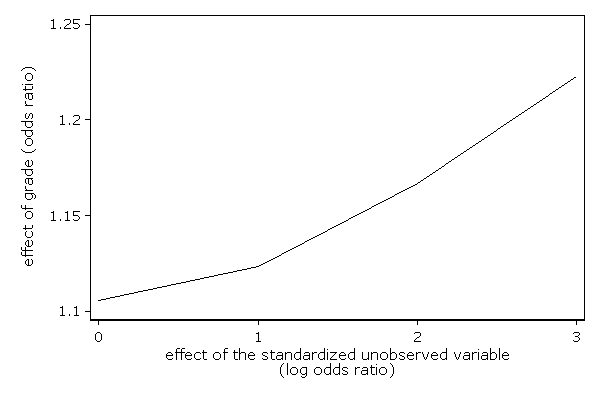
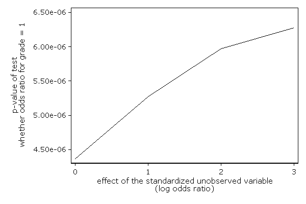
sd or p -------------------------------- 0 1.11 4.37e-06 1 1.12 5.27e-06 2 1.17 5.97e-06 3 1.22 6.28e-06
. . // graph the estimates . // first turn the matrix into variables . svmat res, names(col)
. . // graph the variables . twoway line or sd, /// > xtitle("effect of the standardized unobserved variable" /// > "(log odds ratio)") /// > ytitle("effect of grade (odds ratio)") name(or, replace)
. . twoway line p sd, /// > xtitle("effect of the standardized unobserved variable" /// > "(log odds ratio)") /// > ytitle("p-value of test" /// > "whether odds ratio for grade = 1") name(p, replace)