stdtable
Author: Maarten L. Buis
The purpose of the stdtable command is to describe the association between two categorical variables nett of the association imposed on the table by the marginal distributions or make cross-tabulations comparable across groups by removing differences due to differences in the marginal distributions. The stdtable command does that by standardizing a cross-tabulation by fixing the row and column totals.
This package can be installed by typing in Stata: ssc install stdtable
Example
stdtable standardizes a cross-tabulation such that the by fixing the row and column totals (Yule 1912, Mosteller 1968, Agresti 2002: 345-346). These standardized counts are estimated using Iterative Proportional Fitting. By default it sets all the row and column totals to 100 if the number of columns is the same as the number of rows. Consider the following example from Featherman and Hauser (1978) using data collected in the USA as a supplement to the March Current Population Survey by the U.S. Bureau of the Census in 1973:
. use "http://www.maartenbuis.nl/software/mob.dta", clear (mobility table from the USA collected in 1973)
. notes
_dta: 1. source: Featherman, D.L. and R.M. Hauser (1978) Opportunity and change. New York: Academic.
. codebook, compact
Variable Obs Unique Mean Min Max Label ------------------------------------------------------------------------------- row 25 5 3 1 5 Father's occupation col 25 5 3 1 5 Son's occupation pop 25 25 796.48 40 3325 count -------------------------------------------------------------------------------
. tab row col [fw=pop],
Father's | Son's occupation occupation | upper non lower non upper man lower man farm | Total ----------------+-------------------------------------------------------+---------- upper nonmanual | 1,414 521 302 643 40 | 2,920 lower nonmanual | 724 524 254 703 48 | 2,253 upper manual | 798 648 856 1,676 108 | 4,086 lower manual | 756 914 771 3,325 237 | 6,003 farm | 409 357 441 1,611 1,832 | 4,650 ----------------+-------------------------------------------------------+---------- Total | 4,101 2,964 2,624 7,958 2,265 | 19,912
There are many more people that went from a farm to lower manual than the other way around. However, the number of people in agriculture strongly declined so sons had to leave the farm. Moreover, the number of people in lower manual occupations were on the increase, offering room for those sons that had to leave their farm. We may be interested in knowing if this asymmetry is completely explained by these changes in the marginal distribution, or if there is more to it. We could look at row (outflow) percentages, but than we only control for the distribution of the father's occupation. Similarly, the column (inflow) percentages only control for the distribution of son's occupation. What we want is something that does both simultaneously, i.e. fix both the column totals and the row totals to 100. This is what stdtable does:
. stdtable row col [fw=pop], cellwidth(8)
---------------------------------------------------------------------------- Father's | Son's occupation occupation | upper no lower no upper ma lower ma farm Total ----------------+----------------------------------------------------------- upper nonmanual | 41.7 23.6 17.3 13.1 4.23 100 lower nonmanual | 27 30 18.4 18.1 6.42 100 upper manual | 15.9 19.9 33.2 23.2 7.73 100 lower manual | 11.1 20.6 22 33.8 12.5 100 farm | 4.3 5.78 9.03 11.7 69.1 100 | Total | 100 100 100 100 100 500 ----------------------------------------------------------------------------
These standardized counts can be interpreted as the row and column percentages that would occur if for both fathers and sons each occupation was equally likely. It appears that the apparent asymmetry was almost entirely due to changes in the marginal distributions. Also, it is now much clearer that farming is much more persistent over generations than the other occupations.
This table shows the counts that would have occurred when the odds ratios (effects) are the same as in the data, but the row and column totals were all 100. By setting the row and column totals to all the same number we filter out the effect of the marginal distribution. Setting the row and column totals to a 100 works when we have the same number of rows and columns. If the number of rows and columns differ then the total sample size implied by summing the row totals would not match the total sample size when summing the column totals. In that case the default margins will the 100 / (number of columns) for the column totals and 100 / (number of rows) for row totals. These standardized counts can be interpreted as the cell percentages that would have occurred if each category was equally likely to occur.
Standardizing tables can also be useful to compare tables with different marginal distributions. In the example below we look at the race of husbands and wives in the USA for married couples whose husbands were born born between 1821 and 1989 using the 1880 till 2000 censuses and the 2001 till 2014 American Comunity Surveys. We can see that the racial boundaries have become a bit more permeable over time, but that the USA is still very far removed from being a melting pot.
. use "http://www.maartenbuis.nl/software/interracial.dta", clear (husband's and wife's race in the USA from the census and ACS 1880-2014)
. notes
_dta: 1. Steven Ruggles, Katie Genadek, Ronald Goeken, Josiah Grover, and Matthew Sobek. Integrated Public Use Microdata Series: Version 6.0 [Machine-readable database]. Minneapolis: University of Minnesota, 2015. 2. downloaded on 29 March 2016 from www.ipums.org 3. married persons aged 18-60, unweighted
. codebook, compact
Variable Obs Unique Mean Min Max Label ------------------------------------------------------------------------------- hrace 204 3 2 1 3 husband's race wrace 204 3 2 1 3 wife's race coh 272 17 1900 1820 1980 husband's birth cohort (decade) _freq 272 218 115424.7 0 5632745 Frequency -------------------------------------------------------------------------------
. stdtable hrace wrace [fw=_freq], by(coh)
------------------------------------------ husband's | birth | cohort | (decade) | and | husband's | wife's race race | white black native Total ----------+------------------------------- 1820s | white | 99.3 .119 .561 100 black | .223 99.7 .095 100 native | .457 .199 99.3 100 | Total | 100 100 100 300 ----------+------------------------------- 1830s | white | 99.3 .129 .522 100 black | .276 99.6 .138 100 native | .375 .285 99.3 100 | Total | 100 100 100 300 ----------+------------------------------- 1840s | white | 99.4 .138 .43 100 black | .299 99.5 .153 100 native | .269 .314 99.4 100 | Total | 100 100 100 300 ----------+------------------------------- 1850s | white | 99.6 .21 .235 100 black | .145 99.8 .0647 100 native | .3 0 99.7 100 | Total | 100 100 100 300 ----------+------------------------------- 1860s | white | 99.6 .0782 .287 100 black | .171 99.8 0 100 native | .195 .0924 99.7 100 | Total | 100 100 100 300 ----------+------------------------------- 1870s | white | 99.2 .0868 .761 100 black | .101 99.9 .0483 100 native | .747 .062 99.2 100 | Total | 100 100 100 300 ----------+------------------------------- 1880s | white | 99.2 .123 .68 100 black | .131 99.8 .0798 100 native | .672 .0877 99.2 100 | Total | 100 100 100 300 ----------+------------------------------- 1890s | white | 99 .154 .88 100 black | .105 99.8 .0923 100 native | .929 .0431 99 100 | Total | 100 100 100 300 ----------+------------------------------- 1900s | white | 99 .193 .83 100 black | .194 99.7 .0922 100 native | .829 .0939 99.1 100 | Total | 100 100 100 300 ----------+------------------------------- 1910s | white | 98.8 .232 .965 100 black | .242 99.5 .27 100 native | .955 .28 98.8 100 | Total | 100 100 100 300 ----------+------------------------------- 1920s | white | 97.4 .256 2.36 100 black | .282 99.3 .425 100 native | 2.33 .451 97.2 100 | Total | 100 100 100 300 ----------+------------------------------- 1930s | white | 95.3 .369 4.28 100 black | .425 99.1 .459 100 native | 4.23 .515 95.3 100 | Total | 100 100 100 300 ----------+------------------------------- 1940s | white | 93.1 .713 6.21 100 black | .818 98.5 .64 100 native | 6.1 .745 93.2 100 | Total | 100 100 100 300 ----------+------------------------------- 1950s | white | 92 1.32 6.72 100 black | 1.37 97.8 .846 100 native | 6.67 .897 92.4 100 | Total | 100 100 100 300 ----------+------------------------------- 1960s | white | 91.3 2.2 6.49 100 black | 2.21 96.8 1.02 100 native | 6.49 1.03 92.5 100 | Total | 100 100 100 300 ----------+------------------------------- 1970s | white | 89.9 3.48 6.63 100 black | 3.42 95.3 1.29 100 native | 6.7 1.22 92.1 100 | Total | 100 100 100 300 ----------+------------------------------- 1980s | white | 88.6 4.88 6.53 100 black | 4.77 93.7 1.54 100 native | 6.64 1.43 91.9 100 | Total | 100 100 100 300 ------------------------------------------
The standardized table can be left in memory using the replace option, which can be useful for graphing that table. Nick Cox's tabplot is nice for this.
. qui stdtable hrace wrace [fw=_freq], by(coh) replace
. tabplot hrace coh [iw=std], /// > by(wrace, compact cols(3) note("")) /// > xtitle("husband's birth cohort" "wife's race") /// > xlab(1(2)18,angle(35) labsize(vsmall))
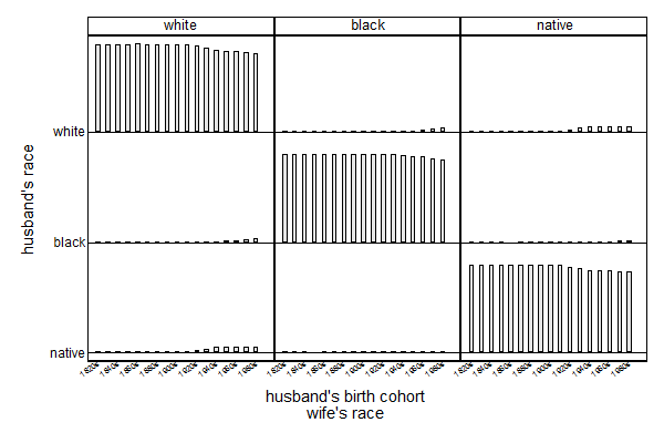
Setting all the row and column totals to a 100 is nice for filtering out the effect for filtering out the effect of the marginal distributions, but is unrealistic. If we just want to filter out the effects of changes in the marginal distributions over time, we could fix all the margins to be equal to the margins of one cohort, say 1980.
. use "http://www.maartenbuis.nl/software/interracial.dta", clear (husband's and wife's race in the USA from the census and ACS 1880-2014)
. stdtable hrace wrace [fw=_freq], by(coh, baseline(1980))
------------------------------------------ husband's | birth | cohort | (decade) | and | husband's | wife's race race | white black native Total ----------+------------------------------- 1820s | white | 723994 13.5 427 724434 black | 5751 39909 256 45916 native | 306 2.07 6951 7259 | Total | 730051 39925 7633 777609 ----------+------------------------------- 1830s | white | 724046 18.1 370 724434 black | 5734 39903 279 45916 native | 271 3.97 6984 7259 | Total | 730051 39925 7633 777609 ----------+------------------------------- 1840s | white | 724114 21 299 724434 black | 5737 39899 280 45916 native | 200 4.87 7054 7259 | Total | 730051 39925 7633 777609 ----------+------------------------------- 1850s | white | 724200 15.5 218 724434 black | 5683 39909 323 45916 native | 167 0 7092 7259 | Total | 730051 39925 7633 777609 ----------+------------------------------- 1860s | white | 723987 6.46 441 724434 black | 5998 39918 0 45916 native | 66.5 .359 7192 7259 | Total | 730051 39925 7633 777609 ----------+------------------------------- 1870s | white | 723851 4.47 579 724434 black | 5710 39920 285 45916 native | 490 .286 6769 7259 | Total | 730051 39925 7633 777609 ----------+------------------------------- 1880s | white | 723931 8.36 494 724434 black | 5658 39916 342 45916 native | 462 .56 6796 7259 | Total | 730051 39925 7633 777609 ----------+------------------------------- 1890s | white | 723832 8.49 594 724434 black | 5548 39916 451 45916 native | 671 .235 6588 7259 | Total | 730051 39925 7633 777609 ----------+------------------------------- 1900s | white | 723783 19.1 632 724434 black | 5728 39905 283 45916 native | 540 .83 6718 7259 | Total | 730051 39925 7633 777609 ----------+------------------------------- 1910s | white | 723805 29.9 599 724434 black | 5504 39891 521 45916 native | 742 3.84 6513 7259 | Total | 730051 39925 7633 777609 ----------+------------------------------- 1920s | white | 722994 39.9 1400 724434 black | 5387 39878 651 45916 native | 1670 6.8 5582 7259 | Total | 730051 39925 7633 777609 ----------+------------------------------- 1930s | white | 721815 85 2534 724434 black | 5612 39830 474 45916 native | 2624 9.72 4625 7259 | Total | 730051 39925 7633 777609 ----------+------------------------------- 1940s | white | 720640 304 3490 724434 black | 5978 39598 339 45916 native | 3433 23 3803 7259 | Total | 730051 39925 7633 777609 ----------+------------------------------- 1950s | white | 719821 858 3754 724434 black | 6600 39026 290 45916 native | 3630 40.5 3588 7259 | Total | 730051 39925 7633 777609 ----------+------------------------------- 1960s | white | 718784 1937 3713 724434 black | 7730 37926 260 45916 native | 3536 62.6 3660 7259 | Total | 730051 39925 7633 777609 ----------+------------------------------- 1970s | white | 716868 3758 3808 724434 black | 9579 36078 259 45916 native | 3604 89 3566 7259 | Total | 730051 39925 7633 777609 ----------+------------------------------- 1980s | white | 714801 5840 3793 724434 black | 11673 33971 272 45916 native | 3577 114 3568 7259 | Total | 730051 39925 7633 777609 ------------------------------------------
References
Agresti, A. (2002) Categorical Data Analysis, second edition. Hoboken: Wiley Interscience.Featherman, D.L. and R.M. Hauser (1978) Opportunity and Change. New York: Academic.
Mosteller, F. (1968) Association and estimation in contingency tables, Journal of the American Statistical Association, 63(321): 1-28.
Yule, U. (1912) On the methods of measuring association between two attributes, Journal of the Royal Statistical Society, 75(6): 579-652.