Additional examples for: Stata tip #: Exploring model consequences by plotting different predictions (Translated to Stata ≥ 12)
Maarten L. BuisTable of content
- Original example
- Adding colors
- Displaying splines instead of quadratic curves
- After logit instead of regress
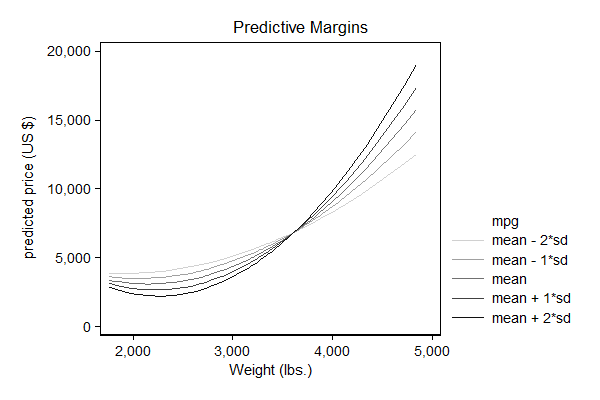
Original example
. * get -lean- scheme . * net install "http://www.stata-journal.com/software/sj4-3/gr0002_3", replace . set scheme lean1
. . // get the data and estimate the model . sysuse auto, clear (1978 Automobile Data)
. qui reg price c.mpg##c.weight##c.weight i.foreign
. . // find values for mpg . qui sum mpg if e(sample)
. forvalues i = -2/2 { 2. local val "`val' `=`r(mean)' + `i'*`r(sd)''" 3. }
. . // get the predictions . qui margins , at( foreign=0 mpg=(`val')) over(weight)
. . // plot the predictions . marginsplot, noci plotopts( msymbol(none) ) /// > xdim(weight) /// > ytitle("predicted price (US {c S|})") /// > ylabel(,format( %8.0gc)) /// > plot1opts(lcolor(gs13)) /// > plot2opts(lcolor(gs10)) /// > plot3opts(lcolor( gs7)) /// > plot4opts(lcolor( gs4)) /// > plot5opts(lcolor( gs1)) /// > legend( order( - "mpg" /// > 1 "mean - 2*sd" /// > 2 "mean - 1*sd" /// > 3 "mean" /// > 4 "mean + 1*sd" /// > 5 "mean + 2*sd" ))
Variables that uniquely identify margins: mpg weight
.
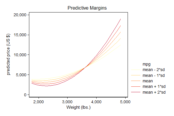
Adding colors
In this application it is useful to choose a gradient of colors for the lines that emphasize the ordinal nature of the predictions. A useful tool that can help choosing such colors is http://colorbrewer2.org/. This will give suggestions for colors in terms of RGB values. You can add these values directly in the Stata graph, as is shown in the example below.
. * get -lean- scheme . * net install "http://www.stata-journal.com/software/sj4-3/gr0002_3", replace . set scheme lean1
. . // get the data and estimate the model . sysuse auto, clear (1978 Automobile Data)
. qui reg price c.mpg##c.weight##c.weight i.foreign
. . // find values for mpg . qui sum mpg if e(sample)
. forvalues i = -2/2 { 2. local val "`val' `=`r(mean)' + `i'*`r(sd)''" 3. }
. . // get the predictions . qui margins , at( foreign=0 mpg=(`val')) over(weight)
. . // plot the predictions . marginsplot, noci plotopts( msymbol(none) ) /// > xdim(weight) /// > ytitle("predicted price (US {c S|})") /// > ylabel(,format( %8.0gc)) /// > plot1opts(lcolor("255 255 178")) /// > plot2opts(lcolor("254 204 92")) /// > plot3opts(lcolor("253 141 60")) /// > plot4opts(lcolor("240 59 32")) /// > plot5opts(lcolor("189 0 38")) /// > legend( order( - "mpg" /// > 1 "mean - 2*sd" /// > 2 "mean - 1*sd" /// > 3 "mean" /// > 4 "mean + 1*sd" /// > 5 "mean + 2*sd" ))
Variables that uniquely identify margins: mpg weight
.
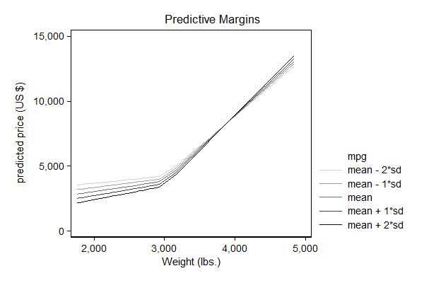
Displaying splines instead of quadratic curves
The idea behind this tip is not limited to quadratic curves, below is an example that applies it to linear splines.
. * get -lean- scheme . * net install "http://www.stata-journal.com/software/sj4-3/gr0002_3", replace . set scheme lean1
. . // get the data and estimate the model . sysuse auto, clear (1978 Automobile Data)
. mkspline w1 3000 w2 = weight
. qui reg price c.mpg##c.w1 c.mpg#c.w2 c.w2 i.foreign
. . // find values for mpg . qui sum mpg if e(sample)
. forvalues i = -2/2 { 2. local val "`val' `=`r(mean)' + `i'*`r(sd)''" 3. }
. . // get the predictions . qui margins , at( foreign=0 mpg=(`val')) over(weight)
. . // plot the predictions . marginsplot, noci plotopts( msymbol(none) ) /// > xdim(weight) /// > ytitle("predicted price (US {c S|})") /// > ylabel(,format( %8.0gc)) /// > plot1opts(lcolor(gs13)) /// > plot2opts(lcolor(gs10)) /// > plot3opts(lcolor( gs7)) /// > plot4opts(lcolor( gs4)) /// > plot5opts(lcolor( gs1)) /// > legend( order( - "mpg" /// > 1 "mean - 2*sd" /// > 2 "mean - 1*sd" /// > 3 "mean" /// > 4 "mean + 1*sd" /// > 5 "mean + 2*sd" ))
Variables that uniquely identify margins: mpg weight
.
After logit instead of regress
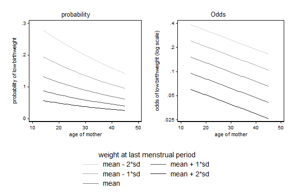
Nor is the idea limited to linear regression or models that include interaction terms. In many non-linear models, like logit, the predictions depend on the baseline value, so that way the effect of one variable will depend on other variables even when no interaction terms was included. However, as is also illustrated below, there is often an alternative way of presenting these effects where this "pseudo-interaction" does not occur.
. * get -lean- scheme . * net install "http://www.stata-journal.com/software/sj4-3/gr0002_3", replace . * . * get -grc1leg- . * net install "http://www.stata.com/users/vwiggins/grc1leg", replace . . set scheme lean1
. . webuse lbw, clear (Hosmer & Lemeshow data)
. qui logit low age lwt i.race smoke ptl ht ui
. . // find values for lwt . qui sum lwt if e(sample)
. local m = r(mean)
. local sd = r(sd)
. . forvalues i = -2/2 { 2. local val "`val' `=`r(mean)' + `i'*`r(sd)''" 3. }
. . // get the predictions . qui margins , at( race=1 smoke=0 ptl=0 ht=0 ui=0 lwt=(`val')) over(age)
. . // plot the predictions . marginsplot, noci plotopts( msymbol(none) ) /// > xdim(age) /// > xlab(10(10)50) /// > name(pr, replace) /// > ytitle("probability of low birthweight") /// > title("probability") /// > plot1opts(lcolor(gs13)) /// > plot2opts(lcolor(gs10)) /// > plot3opts(lcolor( gs7)) /// > plot4opts(lcolor( gs4)) /// > plot5opts(lcolor( gs1)) /// > legend( subtitle("weight at last menstrual period") /// > order( 1 "mean - 2*sd" /// > 2 "mean - 1*sd" /// > 3 "mean" /// > 4 "mean + 1*sd" /// > 5 "mean + 2*sd" ) cols(2) colfirst)
Variables that uniquely identify margins: lwt age
. . // get the predictions . qui margins , at( race=1 smoke=0 ptl=0 ht=0 ui=0 lwt=(`val')) over(age) /// > expression(exp(xb()))
. . marginsplot, noci plotopts( msymbol(none) ) /// > xdim(age) /// > xlab(10(10)50) /// > name(odds, replace) /// > ytitle("odds of low birthweight (log scale)") /// > title("Odds") /// > yscale(log) ylab(.025 .05 .1 .2 .4) /// > plot1opts(lcolor(gs13)) /// > plot2opts(lcolor(gs10)) /// > plot3opts(lcolor( gs7)) /// > plot4opts(lcolor( gs4)) /// > plot5opts(lcolor( gs1)) /// > legend( subtitle("weight at last menstrual period") /// > order( 1 "mean - 2*sd" /// > 2 "mean - 1*sd" /// > 3 "mean" /// > 4 "mean + 1*sd" /// > 5 "mean + 2*sd" ) cols(2) colfirst) >
Variables that uniquely identify margins: lwt age
. . grc1leg pr odds
.