Additional examples for: Stata tip #: Exploring model consequences by plotting different predictions (Translated to Stata < 11)
Maarten L. BuisTable of content
- Original example
- Adding colors
- Displaying splines instead of quadratic curves
- After logit instead of regress
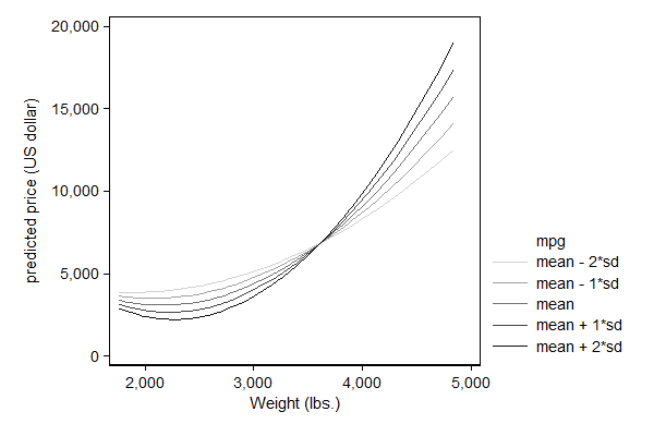
Original example
. * get -lean- scheme . * net install "http://www.stata-journal.com/software/sj4-3/gr0002_3", replace . set scheme lean1
. . sysuse auto, clear (1978 Automobile Data)
. gen weight2 = weight^2
. gen mpgXweight = mpg*weight
. gen mpgXweight2 = mpg*weight2
. reg price mpg weight weight2 mpgXweight mpgXweight2 foreign
Source | SS df MS Number of obs = 74 -------------+------------------------------ F( 6, 67) = 14.35 Model | 357171605 6 59528600.9 Prob > F = 0.0000 Residual | 277893791 67 4147668.52 R-squared = 0.5624 -------------+------------------------------ Adj R-squared = 0.5232 Total | 635065396 73 8699525.97 Root MSE = 2036.6
------------------------------------------------------------------------------ price | Coef. Std. Err. t P>|t| [95% Conf. Interval] -------------+---------------------------------------------------------------- mpg | 339.3687 642.7191 0.53 0.599 -943.504 1622.242 weight | -.4190692 9.351452 -0.04 0.964 -19.08465 18.24651 weight2 | .0003336 .0014293 0.23 0.816 -.0025194 .0031866 mpgXweight | -.3354198 .4546588 -0.74 0.463 -1.242923 .572083 mpgXweight2 | .0000668 .0000766 0.87 0.386 -.0000861 .0002197 foreign | 3169.324 678.0392 4.67 0.000 1815.952 4522.696 _cons | 4005.794 14733.72 0.27 0.787 -25402.84 33414.42 ------------------------------------------------------------------------------
. . qui sum mpg if e(sample)
. local m = r(mean)
. local sd = r(sd)
. . preserve
. qui replace foreign = 0
. . forvalues i = -2/2 { 2. qui replace mpg = `m' + `i'*`sd' 3. qui replace mpgXweight = mpg*weight 4. qui replace mpgXweight2 = mpg*weight2 5. local j = `i' + 2 6. qui predict yhat`j' 7. }
. format yhat* %8.0gc
. sort weight
. twoway line yhat0 yhat1 yhat2 yhat3 yhat4 weight, /// > ytitle("predicted price (US dollar)") /// > clpattern(solid solid solid solid solid) /// > clcolor(gs13 gs10 gs7 gs4 gs1) /// > legend( order( - "mpg" /// > 1 "mean - 2*sd" /// > 2 "mean - 1*sd" /// > 3 "mean" /// > 4 "mean + 1*sd" /// > 5 "mean + 2*sd" ))
. restore
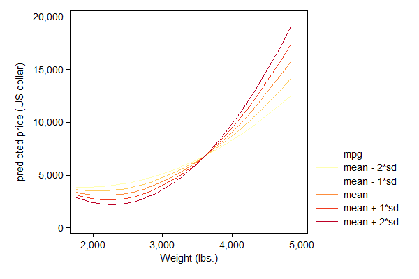
Adding colors
In this application it is useful to choose a gradient of colors for the lines that emphasize the ordinal nature of the predictions. A useful tool that can help choosing such colors is http://colorbrewer2.org/. This will give suggestions for colors in terms of RGB values. You can add these values directly in the Stata graph, as is shown in the example below.
. * get -lean- scheme . * net install "http://www.stata-journal.com/software/sj4-3/gr0002_3", replace . set scheme lean1
. . sysuse auto, clear (1978 Automobile Data)
. gen weight2 = weight^2
. gen mpgXweight = mpg*weight
. gen mpgXweight2 = mpg*weight2
. reg price mpg weight weight2 mpgXweight mpgXweight2 foreign
Source | SS df MS Number of obs = 74 -------------+------------------------------ F( 6, 67) = 14.35 Model | 357171605 6 59528600.9 Prob > F = 0.0000 Residual | 277893791 67 4147668.52 R-squared = 0.5624 -------------+------------------------------ Adj R-squared = 0.5232 Total | 635065396 73 8699525.97 Root MSE = 2036.6
------------------------------------------------------------------------------ price | Coef. Std. Err. t P>|t| [95% Conf. Interval] -------------+---------------------------------------------------------------- mpg | 339.3687 642.7191 0.53 0.599 -943.504 1622.242 weight | -.4190692 9.351452 -0.04 0.964 -19.08465 18.24651 weight2 | .0003336 .0014293 0.23 0.816 -.0025194 .0031866 mpgXweight | -.3354198 .4546588 -0.74 0.463 -1.242923 .572083 mpgXweight2 | .0000668 .0000766 0.87 0.386 -.0000861 .0002197 foreign | 3169.324 678.0392 4.67 0.000 1815.952 4522.696 _cons | 4005.794 14733.72 0.27 0.787 -25402.84 33414.42 ------------------------------------------------------------------------------
. . qui sum mpg if e(sample)
. local m = r(mean)
. local sd = r(sd)
. . preserve
. qui replace foreign = 0
. . forvalues i = -2/2 { 2. qui replace mpg = `m' + `i'*`sd' 3. qui replace mpgXweight = mpg*weight 4. qui replace mpgXweight2 = mpg*weight2 5. local j = `i' + 2 6. qui predict yhat`j' 7. }
. format yhat* %8.0gc
. sort weight
. twoway line yhat0 yhat1 yhat2 yhat3 yhat4 weight, /// > ytitle("predicted price (US dollar)") /// > clpattern(solid solid solid solid solid) /// > clcolor("255 255 178" /// > "254 204 92" /// > "253 141 60" /// > "240 59 32" /// > "189 0 38") /// > legend( order( - "mpg" /// > 1 "mean - 2*sd" /// > 2 "mean - 1*sd" /// > 3 "mean" /// > 4 "mean + 1*sd" /// > 5 "mean + 2*sd" ))
. restore
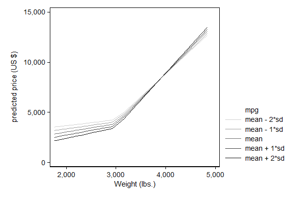
Displaying splines instead of quadratic curves
The idea behind this tip is not limited to quadratic curves, below is an example that applies it to linear splines.
. * get -lean- scheme . * net install "http://www.stata-journal.com/software/sj4-3/gr0002_3", replace . set scheme lean1
. . sysuse auto, clear (1978 Automobile Data)
. mkspline w1 3000 w2 = weight
. gen mpgXw1 = mpg*w1
. gen mpgXw2 = mpg*w2
. reg price mpg w1 w2 mpgXw1 mpgXw2 foreign
Source | SS df MS Number of obs = 74 -------------+------------------------------ F( 6, 67) = 13.75 Model | 350442579 6 58407096.5 Prob > F = 0.0000 Residual | 284622817 67 4248101.75 R-squared = 0.5518 -------------+------------------------------ Adj R-squared = 0.5117 Total | 635065396 73 8699525.97 Root MSE = 2061.1
------------------------------------------------------------------------------ price | Coef. Std. Err. t P>|t| [95% Conf. Interval] -------------+---------------------------------------------------------------- mpg | -95.44225 385.0294 -0.25 0.805 -863.9641 673.0796 w1 | .3707357 3.900715 0.10 0.925 -7.415124 8.156595 w2 | 4.231955 2.964785 1.43 0.158 -1.68578 10.14969 mpgXw1 | .0205254 .1642997 0.12 0.901 -.3074183 .3484691 mpgXw2 | .0372192 .1768719 0.21 0.834 -.3158184 .3902569 foreign | 3178.442 687.4848 4.62 0.000 1806.217 4550.668 _cons | 3462.536 9888.378 0.35 0.727 -16274.75 23199.82 ------------------------------------------------------------------------------
. . qui sum mpg if e(sample)
. local m = r(mean)
. local sd = r(sd)
. . preserve
. qui replace foreign = 0
. . forvalues i = -2/2 { 2. qui replace mpg = `m' + `i'*`sd' 3. qui replace mpgXw1 = mpg*w1 4. qui replace mpgXw2 = mpg*w2 5. local j = `i' + 2 6. qui predict yhat`j' 7. }
. format yhat* %8.0gc
. sort weight
. twoway line yhat0 yhat1 yhat2 yhat3 yhat4 weight, /// > ytitle("predicted price (US {c S|})") /// > clpattern(solid solid solid solid solid) /// > clcolor(gs13 gs10 gs7 gs4 gs1) /// > legend( order( - "mpg" /// > 1 "mean - 2*sd" /// > 2 "mean - 1*sd" /// > 3 "mean" /// > 4 "mean + 1*sd" /// > 5 "mean + 2*sd" ))
. restore
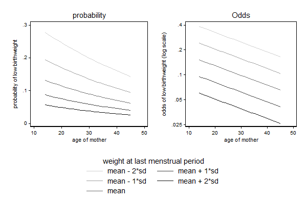
After logit instead of regress
Nor is the idea limited to linear regression or models that include interaction terms. In many non-linear models, like logit, the predictions depend on the baseline value, so that way the effect of one variable will depend on other variables even when no interaction terms was included. However, as is also illustrated below, there is often an alternative way of presenting these effects where this "pseudo-interaction" does not occur.
. * get -lean- scheme . * net install "http://www.stata-journal.com/software/sj4-3/gr0002_3", replace . * . * get -grc1leg- . * net install "http://www.stata.com/users/vwiggins/grc1leg", replace . . set scheme lean1
. . webuse lbw, clear (Hosmer & Lemeshow data)
. xi: logit low age lwt i.race smoke ptl ht ui i.race _Irace_1-3 (naturally coded; _Irace_1 omitted)
Iteration 0: log likelihood = -117.336 Iteration 1: log likelihood = -101.28644 Iteration 2: log likelihood = -100.72617 Iteration 3: log likelihood = -100.724 Iteration 4: log likelihood = -100.724
Logistic regression Number of obs = 189 LR chi2(8) = 33.22 Prob > chi2 = 0.0001 Log likelihood = -100.724 Pseudo R2 = 0.1416
------------------------------------------------------------------------------ low | Coef. Std. Err. z P>|z| [95% Conf. Interval] -------------+---------------------------------------------------------------- age | -.0271003 .0364504 -0.74 0.457 -.0985418 .0443412 lwt | -.0151508 .0069259 -2.19 0.029 -.0287253 -.0015763 _Irace_2 | 1.262647 .5264101 2.40 0.016 .2309024 2.294392 _Irace_3 | .8620792 .4391532 1.96 0.050 .0013548 1.722804 smoke | .9233448 .4008266 2.30 0.021 .137739 1.708951 ptl | .5418366 .346249 1.56 0.118 -.136799 1.220472 ht | 1.832518 .6916292 2.65 0.008 .4769494 3.188086 ui | .7585135 .4593768 1.65 0.099 -.1418484 1.658875 _cons | .4612239 1.20459 0.38 0.702 -1.899729 2.822176 ------------------------------------------------------------------------------
. . qui sum lwt if e(sample)
. local m = r(mean)
. local sd = r(sd)
. . preserve
. qui replace _Irace_2 = 0
. qui replace _Irace_3 = 0
. qui replace smoke = 0
. qui replace ptl = 0
. qui replace ht = 0
. qui replace ui = 0
. . forvalues i = -2/2 { 2. qui replace lwt = `m' + `i'*`sd' 3. local j = `i' + 2 4. qui predict pr`j' 5. qui predict odds`j', xb 6. qui replace odds`j' = exp(odds`j') 7. }
. format pr* %8.0gc
. sort age
. twoway line pr0 pr1 pr2 pr3 pr4 age, /// > name(pr, replace) /// > ytitle("probability of low birthweight") /// > title("probability") /// > clpattern(solid solid solid solid solid) /// > clcolor(gs13 gs10 gs7 gs4 gs1) /// > legend( subtitle("weight at last menstrual period") /// > order( 1 "mean - 2*sd" /// > 2 "mean - 1*sd" /// > 3 "mean" /// > 4 "mean + 1*sd" /// > 5 "mean + 2*sd" ) cols(2) colfirst)
. . twoway line odds0 odds1 odds2 odds3 odds4 age, /// > name(odds, replace) /// > ytitle("odds of low birthweight (log scale)") /// > title("Odds") /// > yscale(log) ylab(.025 .05 .1 .2 .4) /// > clpattern(solid solid solid solid solid) /// > clcolor(gs13 gs10 gs7 gs4 gs1) /// > legend( subtitle("weight at last menstrual period") /// > order( 1 "mean - 2*sd" /// > 2 "mean - 1*sd" /// > 3 "mean" /// > 4 "mean + 1*sd" /// > 5 "mean + 2*sd" ) cols(2) colfirst)
. . grc1leg pr odds
. . restore