oparallel
Author: Maarten L. Buis
oparallel is a post-estimation command testing the parallel regression assumption in a ordered logit model. By default it performs five tests: a likelihood ratio test, a score test, a Wald test, a Wolfe-Gould test, and a Brant test. These tests compare a ordered logit model with the fully generalized ordered logit model, which relaxes the parallel regression assumption on all explanatory variables. Optionally, oparallel can use the bootstrap to compute the p-values for these tests. A discussion of these tests was given in a presentation at the 13th German Stata Users' group meeting. The slides of that talk can be downloaded here.
This package can be installed by typing in Stata: ssc install oparallel
Examples
A basic example
. use "http://www.indiana.edu/~jslsoc/stata/spex_data/ordwarm2.dta", clear (77 & 89 General Social Survey)
. ologit warm white ed prst age
Iteration 0: log likelihood = -2995.7704 Iteration 1: log likelihood = -2913.6651 Iteration 2: log likelihood = -2913.2245 Iteration 3: log likelihood = -2913.2244
Ordered logistic regression Number of obs = 2293 LR chi2(4) = 165.09 Prob > chi2 = 0.0000 Log likelihood = -2913.2244 Pseudo R2 = 0.0276
------------------------------------------------------------------------------ warm | Coef. Std. Err. z P>|z| [95% Conf. Interval] -------------+---------------------------------------------------------------- white | -.4478496 .1181476 -3.79 0.000 -.6794147 -.2162845 ed | .078407 .0158339 4.95 0.000 .0473731 .1094408 prst | .0053391 .0032788 1.63 0.103 -.0010872 .0117654 age | -.0186559 .002439 -7.65 0.000 -.0234362 -.0138756 -------------+---------------------------------------------------------------- /cut1 | -2.056959 .2334583 -2.514529 -1.59939 /cut2 | -.2866278 .2287289 -.7349282 .1616727 /cut3 | 1.525569 .2308303 1.07315 1.977989 ------------------------------------------------------------------------------
. oparallel
Tests of the parallel regression assumption
| Chi2 df P>Chi2 -----------------+---------------------- Wolfe Gould | 14.61 8 0.067 Brant | 15.96 8 0.043 score | 14.93 8 0.061 likelihood ratio | 14.75 8 0.064 Wald | 15.08 8 0.058
Computing bootstrap p-values for the Brant test. The bootstrap p-values (ASL) is close to the asymptotic one (P>Chi2), but the uncertainty due to the randomness in the bootstrap procedure is large enough that the Monte Carlo confidence interval (95% MC CI) does still include 5%.
. use "http://www.indiana.edu/~jslsoc/stata/spex_data/ordwarm2.dta", clear (77 & 89 General Social Survey)
. qui ologit warm white ed prst age
. oparallel, brant asl mcci nodots
Test of the parallel regression assumption
| Chi2 df P>Chi2 ASL [95% MC CI] -----------------+--------------------------------------------- Brant | 15.96 8 0.043 0.048 0.036 0.062
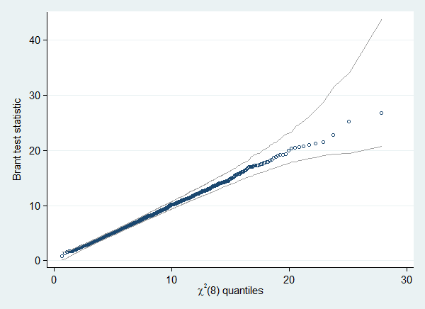
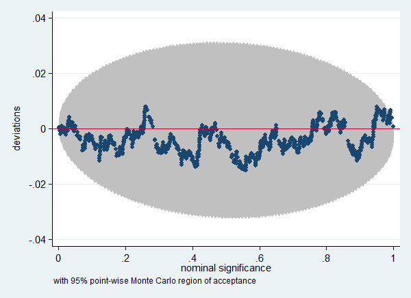
The distribution of the test statistics from the different bootstrap replications is an estimate of the sampling distribution of that statistic if the null hypothesis is true. You can save the test statistics using the saving() option, and check if that distribution corresponds with the theoretical distribution; a Chi-square distribution for the test statistic and a standard uniform distribution for the p-values. In this case the Brant test seems to perform well. Situations where these tests are likely to fail are discussed here.
This example requires the qenv, qplot, and simpplot packages.
. use "http://www.indiana.edu/~jslsoc/stata/spex_data/ordwarm2.dta", clear (77 & 89 General Social Survey)
. qui ologit warm white ed prst age
. tempfile reps
. oparallel, brant asl saving(`reps') nodots
Test of the parallel regression assumption
| Chi2 df P>Chi2 ASL -----------------+----------------------------- Brant | 15.96 8 0.043 0.046
. use `reps', clear
. . qenvchi2 Brant_stat, gen(lb ub) df(8) overall reps(5000)
. qplot Brant_stat lb ub, ms(oh none ..) c(. l l) /// > lc(gs10 ..) legend(off) ytitle("Brant test statistic") /// > trscale(invchi2(8,@)) xtitle("{&chi}{sup:2}(8) quantiles") /// > scheme(s2color) ylab(,angle(horizontal))
. . simpplot Brant_p, scheme(s2color) ylab(,angle(horizontal))